Tokyo/Formulation/5.stochastic differential equation model with poisson random variables

From 2007.igem.org

Revision as of 09:11, 24 October 2007

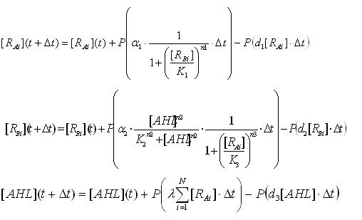
we introduced the terms of Ex 4-1 into a stochastic process to simulate the sthochastic behavior.we used Poisson random variables as a sthochastic process. Threfore,a stochastic differential equations were given as

Ex 5-1

Table 5

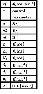
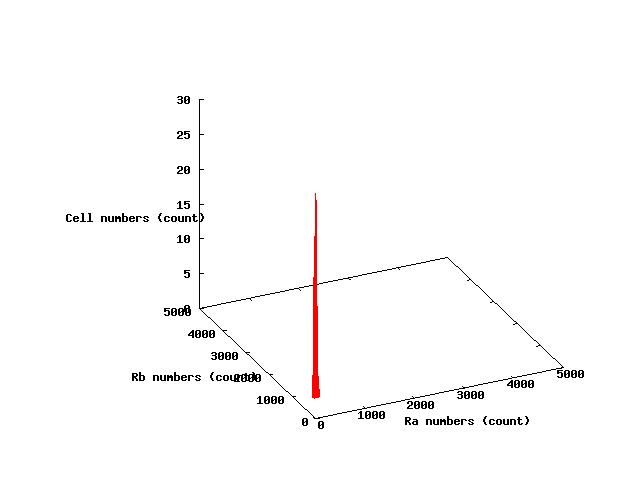
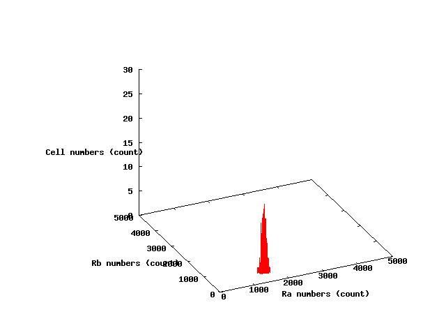
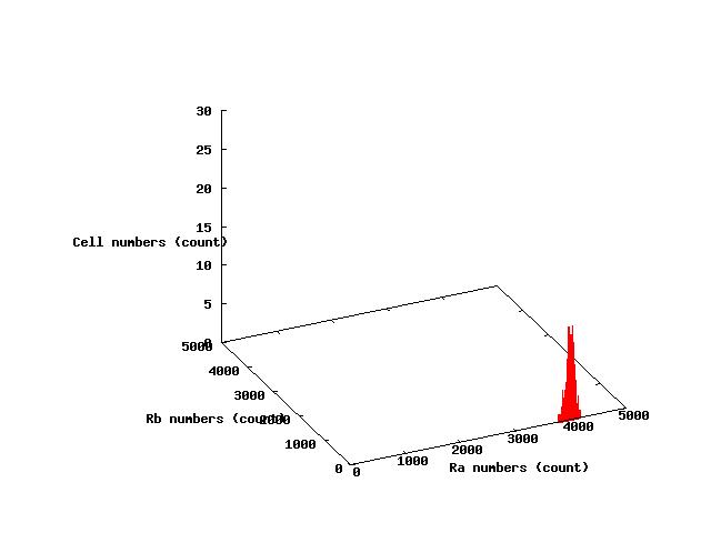
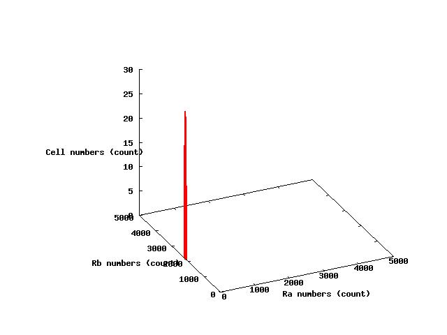
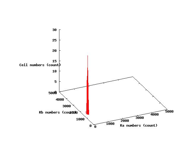
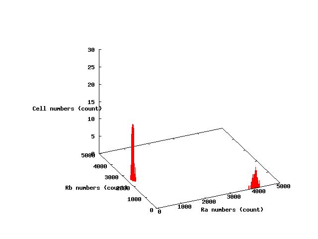
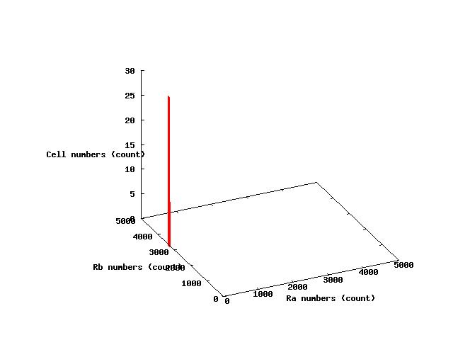
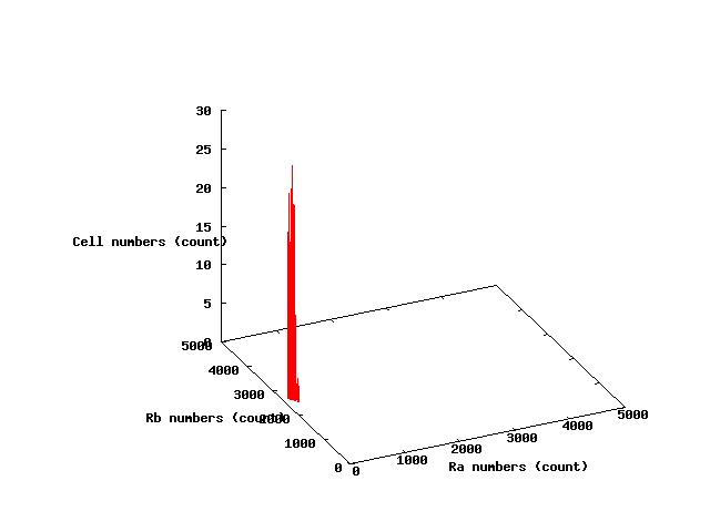
The values of parameters in the right table were used and the results of simulation were shown in Fig 5.1-3.
where α2 = 1(μM) in Fig 5.1,α2 = 2.7(μM) in Fig 5.2,α2 = 4(μM) in Fig 5.3. and it has been estimated that 1(μM) = 1000 molecules (count).

Figure 5.1.A 　t=0.2(min)

Figure 5.1.B 　t=0.8(min)

Figure 5.1.C 　 t=30(min)　　 failure only A

Figure 5.2.A 　t=0.2(min)

Figure 5.2.B 　 t=0.8(min)

Figure 5.2.C 　 t=30(min)　　success!! coexistence

Figure 5.3.A 　 t=0.2(min)

Figure 5.3.B 　 t=0.8(min)

Figure 5.3.C 　 t=30(min)　　 failure only B

パラメータを３種類使ってシミュレーションした結果が以下である． これとstep4のdetermineの相平面とを比べるとこうですよ．