Modelling
From 2007.igem.org
| (12 intermediate revisions not shown) | |||
| Line 1: | Line 1: | ||
===Mathematical Modelling=== | ===Mathematical Modelling=== | ||
| - | To create a predictive model, we used | + | To create a predictive model, we used ordinary differential equations (ODEs) to characterize the concentrations of each protein with respect to time. The general form of the ODEs is shown below, with basal expression of a protein, Hill function describing gene regulation and protein decay [1]. |
| - | + | ||
| + | |||
[[Image:UW_equation.jpg|300px|center]] | [[Image:UW_equation.jpg|300px|center]] | ||
| - | [[Image:UW_Graphs.png|thumb|center|800px| | + | |
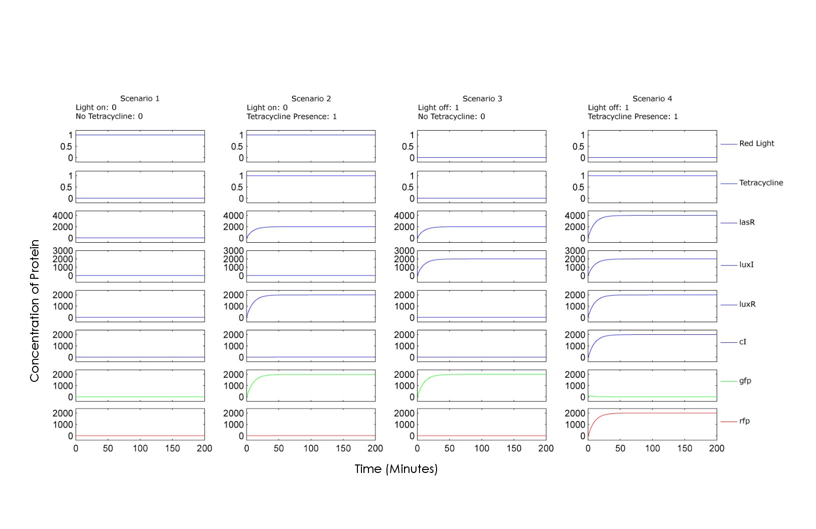
| + | The model is simulated in MATLAB. The following graphs are the simulation results, showing the relative concentrations of proteins involved for each possible combination of input A and input B, red light and tetracycline respectively. Scenario 1 of the graph illustrates the concentration of chemicals when adding 0+0, showing no production of either GFP or RFP. Scenario 2 illustrates the 0+1 case, showing production of GFP. Similarly, scenario 3 illustrates the 1+0 case, also resulting in GFP. Finally, scenario 4 illustrates 1+1 case where the "on" state of both inputs results in production of RFP. | ||
| + | |||
| + | |||
| + | |||
| + | [[Image:UW_Graphs.png|thumb|center|800px|Simulation results of the bacterial half-adder]] | ||
| + | |||
| + | |||
| + | |||
| + | [1] Z. Szallasi, V. Periwal, J. Stelling (eds), ''System Modeling in Cellular Biology: From Concepts to Nuts and Bolts'', MIT Press, Cambridge, MA, 125-148, 2006. | ||
| + | |||
| + | <center> | ||
| + | [[Waterloo | Home ]] | [[Project | Project]] | [[Modelling | Mathematical Modelling]] | [[Construction_and_Testing | Construction and Testing]] | [[Future_Work | Future Work]] | ||
| + | </center> | ||
Latest revision as of 03:18, 27 October 2007
Mathematical Modelling
To create a predictive model, we used ordinary differential equations (ODEs) to characterize the concentrations of each protein with respect to time. The general form of the ODEs is shown below, with basal expression of a protein, Hill function describing gene regulation and protein decay [1].
The model is simulated in MATLAB. The following graphs are the simulation results, showing the relative concentrations of proteins involved for each possible combination of input A and input B, red light and tetracycline respectively. Scenario 1 of the graph illustrates the concentration of chemicals when adding 0+0, showing no production of either GFP or RFP. Scenario 2 illustrates the 0+1 case, showing production of GFP. Similarly, scenario 3 illustrates the 1+0 case, also resulting in GFP. Finally, scenario 4 illustrates 1+1 case where the "on" state of both inputs results in production of RFP.
[1] Z. Szallasi, V. Periwal, J. Stelling (eds), System Modeling in Cellular Biology: From Concepts to Nuts and Bolts, MIT Press, Cambridge, MA, 125-148, 2006.
Home | Project | Mathematical Modelling | Construction and Testing | Future Work

