Valencia/Silico Work
From 2007.igem.org
| Line 12: | Line 12: | ||
When we try to develop a model of this system, we can try to develop a kinetic model in which all the species involved in the model are described. In that kind of model, we consider first the biochemical equations of that system that can be written in the following way: | When we try to develop a model of this system, we can try to develop a kinetic model in which all the species involved in the model are described. In that kind of model, we consider first the biochemical equations of that system that can be written in the following way: | ||
| - | [[image: | + | |
| + | [[image:V1Eq.jpg]] | ||
| + | |||
where Pi are products and ni its mol number, then Rj and mj the same for reactives. Thus, using kinetic constants we can write differential equations. This equations are not much complicated, as they are in first order; but they are non-linear. | where Pi are products and ni its mol number, then Rj and mj the same for reactives. Thus, using kinetic constants we can write differential equations. This equations are not much complicated, as they are in first order; but they are non-linear. | ||
| - | [[image: | + | |
| + | [[image:V2Eq.jpg]] | ||
| + | |||
The problem with this strategy is that usually to know the value of the kinetic constants is quite complicated, as a consequence of that at the we decided to simulate de behaviour of the system using the effective model that we are going to describe later on. | The problem with this strategy is that usually to know the value of the kinetic constants is quite complicated, as a consequence of that at the we decided to simulate de behaviour of the system using the effective model that we are going to describe later on. | ||
Revision as of 15:56, 28 September 2007


|
|
Contents |
Constructing our model
Introduction
The most important part of the theory is to have a good model which represents the real behaviour of the system. Of course all the mathematical models will be an idealization of the biological reality. The aim of this theoretical part, is to develop a qualitative analysis of the expected response of our system. This analysis could be useful to find unexpected behaviours, like chaotical or oscillatory ones, and to search solutions for those possible problems. To do that, we will study the stable solutions, and its stability.
When we try to develop a model of this system, we can try to develop a kinetic model in which all the species involved in the model are described. In that kind of model, we consider first the biochemical equations of that system that can be written in the following way:
where Pi are products and ni its mol number, then Rj and mj the same for reactives. Thus, using kinetic constants we can write differential equations. This equations are not much complicated, as they are in first order; but they are non-linear.
The problem with this strategy is that usually to know the value of the kinetic constants is quite complicated, as a consequence of that at the we decided to simulate de behaviour of the system using the effective model that we are going to describe later on.
Choosing the variables
We are going to work supposing that the variables are continuous. This hypothesis is based in the fact that the variables represent the concentration of proteins, and in the system there will be thousands of them, so having one protein more or one less, will produce a differential variation of the variable. Whenever we can express smalls variations with a differential, and not an increment, we say that the variable is continuous, like in our case.
The equations
We have two ways of describing the actuation of a given protein, we will call it Activator or Repressor. Both actuations are complementary, acting like a switch. We are going to study them before using them in our model.
Activator
The activator works like a switch on system, when the concentration of X arises, the concentration of Y grows too. The relation between both variables is not linear; we want a behavior in which Y has a fast increase with variations of X in a certain interval, and stable outside that interval. The curve of that process is called sigmoid, and it regulates the responses in several biological process. There are a lot of functions that represents this curve, but we have chosen the following:
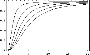
In this function, there are two constants which modify the apparency of the curve, variating its position and its slope. The k constant, sets the position of the curve variating its middle point. In this graph we can see an example of that variation. We set n = 2 and change k in the interval of [1, 5] by steps of 1.
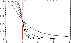
The constant n, called the Hill coefficient, changes the slope of the curve making its slope more or less steeper. When the Hill coefficient is high, the curve is like a step. In the limit of ![]() , the function becomes the Heaviside function or Step Function. In the following graph we can see that process when the value of n is changed, remaining k constant.
, the function becomes the Heaviside function or Step Function. In the following graph we can see that process when the value of n is changed, remaining k constant.
Repressor
We could call the Repressor the inverse function of the Activator. It works like the activator, but stopping the production of the protein Y: in presence of X, the production of Y goes down. Like in the Activator we want that with a short variation of X we obtain a quick stop of the production of Y. The following functions represents that behaviour:
Like in the activator, there are two constants which values determine the shape of the curve, the constant k and the Hill coefficient. We can see the repressor function in the next graph.
The first approach to the model
The dynamical equations
To start with, we must construct the equations which will represent the dynamical process of the model. Let there be a protein X, the input , and protein Y, the output. We want to study how the response of the production of Y in the presence of X will be. We will represent the time-dependent variation of the concentration of the protein Y with a function F which will depend of the concentration of X, the concentration of Y and perhaps of the time t.
The relation of the variation of Y and the concentration of X is known: the Repressor function. We must include an undetermined constant of proportionality α relating the function with the variation. Supposing an initial concentration of protein Y, its variation with time will be a degradation according to the decay law, so there will be a linear relation between the variation of Y and how much proteins there are left. It will have a decay constant β that will be the half-life of the protein, with a minus sign because it is a decay rate. In the cell there could be a basal production of the protein Y, which we will represent with a constant γ. With that analysis, we could construct a final dynamic equation which take into account those relationships between constants and variables.
As a summary, it should be suitable to give now a biological meaning for all the constants:
- α has the information of transcription and translation, this is the rate synthesis
- β has the degradation information
- γ is the basal synthesis, this is a low value
- K is the threshold to protein concentration, namely, it has information about the binding between repressors/activators and promoters
- n is the Hill coefficient (regulation by monomer, dimer, trimer), which has the information about the transitions between two states, it measures the slope of the response
The dynamical system
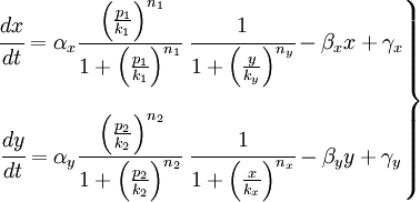
We have studied the equation that involves the dynamical behavior of a repressed protein. But we must build a model in which two proteins repress each other. So we will have two coupled equations which represents the system's behaviour. Each equation will have its own set of constants. We will denote with a subindex the constants of each equation. Finally we can describe the system as:
This is the system of differential equations that we must solve. We can see that it's a highly non-linear system, so we should solve it by numerical methods.
Choosing the constants
One of the most delicate step in this process, is to choose a correct joint of constants which fits correctly to the biological reality. To start with, we will need a reference point to initialize our variables. The principal support in the election of the variables was the well-know article of Elowitz and Leiber, A synthetic oscillatory network of transcriptional regulators1. In this article the use three genes which are repressed one each other. Two of that genes are going to be used by us, so the constants that they used in their theoretical work could be a good start point in our model. We must cite here the part of the article that talks about the constants:
“...average translation efficiency, 20 proteins per transcript, Hill coefficient, n = 2; protein halflife, 10 min; mRNA half-life, 2 min; K, 40 monomers per cell.”
We can get some useful information about the constants: α = 20, n = 2, k = 40, and β should be Ln (2) over the half-life in minutes; so β = 0.069
The dynamical analysis
Numerical simulation of the dynamical system
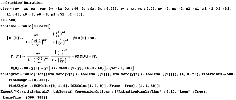
Now we have all the ingredients to make a first simulation of our system. This system is a non-linear system because the dynamical variables involved in the process like x and y, appear in functions that aren't linear, like the repressor one. So the resolution of the system should be made by numerical methods. We will use me mathematical program Mathematica2 to develop our analysis.
First of all we include the set of constants that we will use in the process. After that we include the command NDSolve to resolve a differential equation system by numerical methods. Then we must include two important constants which will decide the final state of the system. They are the initial concentration of x and y; which will be denoted by x0 and y0.
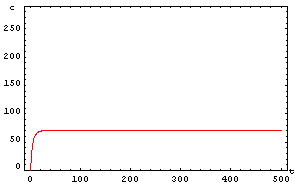
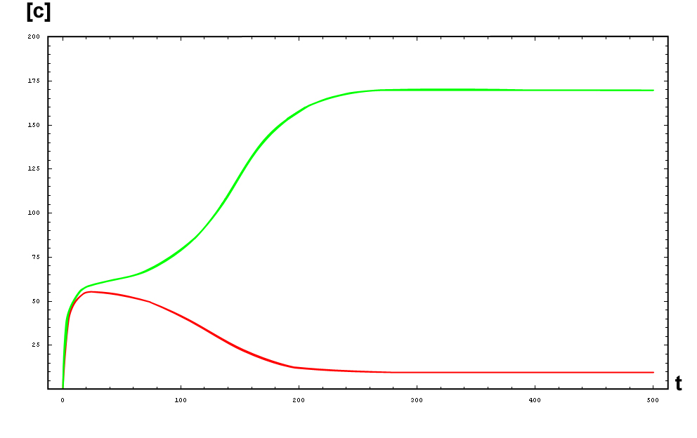
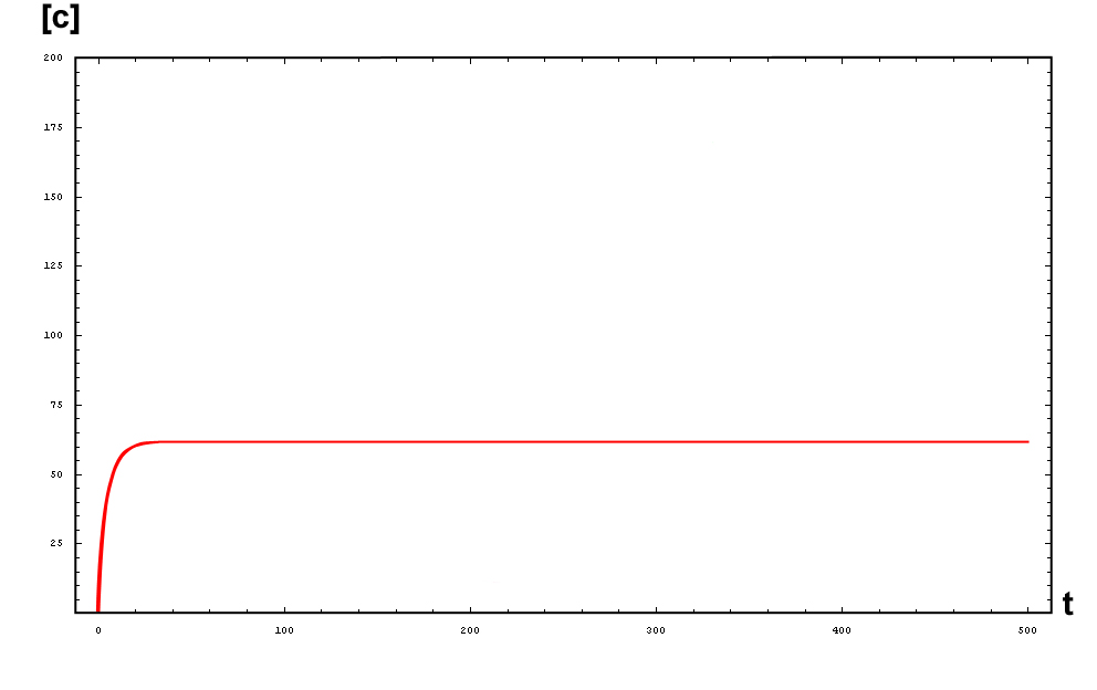
The protein concentration which begins with the highest level will be the ”winner”. So if x0 = 0.5 and y0=0.1, the final and stable state will be x with a high concentration and y with a despicable concentration. In the next graphs we can see that: in the first one x0 is grater than y0 so the stable state is x high (green) and y very low (red). In the second one y0 is greater than x0 and we have the opposite estate. The last one is the unstable state with both variables with the same initial value.
Checking the stability of the system
Now we must test the stability of the steady states. To do that, we have to evaluate the eigenvalues of the Jacobian matrix of the system. First of all, we need to obtain the values of X and Y in the steady state. In that point of the system, there isn't evolution of the system, so the variables X and Y are constants.
That is a system with two equations and two variables that we can solve and obtain xest and yest. To construct the Jacobian matrix we must derivate each function with each constant, and then evaluate the derivate in xest and yest.
We will obtain a 2x2 matrix easily diagonalizable. If the all eigenvalues have the real part negative, the state for that xest and yest is stable.
Example
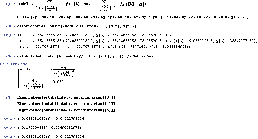
With the aim to understand the last process explained, we are going to develop an example of how to check the stability of the system. First of all we must define the system and its variables. After that the program solve the system in an stationary state, finding five solutions: the two first are complex, so they aren't valid, the others are the solutions of the graphs of the last section: in one win the protein X, in other the Y and in the other there was a draw. We keep that solution in the array “estacionarias”.
Then we determinate the Jacobian matrix and evaluate each solution to obtain the eigenvalues of the matrix. We find that in the case when a protein win, it's a stable state; but the draw case is an unstable state. That means that a little variation in that state, will collapse in one of the others.
You can take a look at the Mathematica file of that example:[http://www.igem.upv.es/igem07/images/3/37/EstabilidadWiki.rar Stability] (Right click and choose "Save as")
The Next Step: The Promoters
The promoters as activators
The have just studied the part of our project that works like a black box but we need the inputs. In that section we are going to include the action of the promoters in our model. You can see in the idea, that we will have two promoters: promoter 1 and promoter 2: p1 and p2 respectively. The p1 actives the production of X and p2 the production of Y. So we will use the promoters like the activators of the proteins. The system will be like that:
In that system we must include the constants of the activator function for each promoter; k and n. The final state of our system will not depend on the initial concentrations of X and Y, but not of the concentrations of the promoters, which should be something we could control.
So, here we have an example of how is the dynamical of the system with the promoters. In that case the initial concentrations of p1 and p2 determinate the behavior of the system. Let see some examples:
From this figures, it is straightforward that the system changes radically its final response according the relative values of p1 and p2.
The promoter as dynamical variable
In the last section we had omitted one important characteristic of the system: the promoters can be treated as a dynamical variable. The only possible process involved in a variation of the promoters, is the disintegration of the proteins. So we should include two more equations at the system, one for each promoter.
That is a very simple equation which solution is know: an exponential.
Where pi0 its the initial concentration of the promoter and βi its the decay constant. If the half-life its higher that our time of measure, we could consider the promoters constants like in the last section. We can see that if the half-life is hight implies that the decay constant its small, so:
Checking the Variables
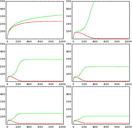
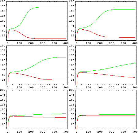
Now is time to take a review of our constants and check how depends the stability and results of the system modifying the value of the constants. The easiest way is to evaluate the system for each value of the constant in a range of interest. For example, we had initialized the value of α at 20, so we could analyze the system in the range from 1 to 30 (we omitted the zero because α = 0 it is a trivial system).
The procedure is simple: we take one value of α and solve the system; after that we increment the value of α and solve again the equations system. The keep the plots in an array, and then we animate the joint of graphs and save it in a GIF file.
The next animations represents how the dynamic of the system changes variating the constants.
The Ecolibrator
The Ecolibrator is a bacteria able to measure the relative strenght of a promoter compared to the streght of a defined promoter known as pattern. In that way, it could generate a scale to define the strenght of several promoters.
References
- Elowitz, Michael B; Leibler, Stanislas, A synthetic oscillatory network of transcriptional regulators, 2000, Nature, 403,6767, p. 335 [http://www.nature.com/nature/journal/v403/n6767/pdf/403335a0.pdf]
- Wolfram Research, Mathematica® Version 5.2 [http://www.wolfram.com/ Web page]


