Glasgow/Modeling
From 2007.igem.org
(→BioBrick library) |
(→Petri Net Modelling) |
||
| Line 169: | Line 169: | ||
= Petri Net Modelling = | = Petri Net Modelling = | ||
| + | [[Image: Glasgow_petri.png|400px|right]] | ||
[http://en.wikipedia.org/wiki/Petri_nets Petri nets] are used to describe discrete distributed systems that | [http://en.wikipedia.org/wiki/Petri_nets Petri nets] are used to describe discrete distributed systems that | ||
have concurrent processes, and provide users with an intuitive | have concurrent processes, and provide users with an intuitive | ||
| Line 200: | Line 201: | ||
To see the full PDF report on Minicap [[https://static.igem.org/mediawiki/2007/f/fb/Minicap.pdf click here]]. | To see the full PDF report on Minicap [[https://static.igem.org/mediawiki/2007/f/fb/Minicap.pdf click here]]. | ||
| - | |||
| - | |||
= BioBrick library = | = BioBrick library = | ||
Revision as of 14:58, 18 October 2007
| https://static.igem.org/mediawiki/2007/thumb/c/cc/Uog.jpg/50px-Uog.jpg | Back To Glasgow's Main Page | Go To Glasgow's Wetlab Log |
|---|
| Modelling | Log | Tutorials | References |
Contents |
Summary
Synthetic biology has been used to describe an approach to biology which attempts to design and construct deliberate biological systems that can be investigated experimentally, which are otherwise very expensive and practically challenging. One of the central features of synthetic biology is the appreciation of the knowledge from science and engineering disciplines for the better design and understanding of synthetic networks. Here we have engineered a bacterial biosensor with the involvement of the construction of two new reporter genes PhzM and PhzS to detect polluting chemicals, which has the potential to provide an inexpensive and easy-to-use method of detecting industrial pollution. We explored a variety of computational approaches to study the behaviour of three synthetic systems: simple reporter system, positive feedback reporter system and [...]. We developed deterministic and stochastic models that quantitatively describe the graded signal-response property of the simple reporter system, and also showed that models can be expanded and used to qualitatively predict the in vivo behaviour of the complicated systems. The dynamics is further studied via the application of qualitative modelling methods. Simulations reveal that the model with positive feedback loop has higher output level than that from the intact model [...] This work shows that by integrating engineering techniques with scientific methodologies, we can gain a new insights into the genetic regulation and should become the reference framework for the design and construction of biochemical networks in synthetic biology.
Framework
We have used a framework which unifies the qualitative, stochastic and continuous worlds, as a basis for our overall approach to modelling and analysing the biochemical pathways. Each perspective adds its contribution to the understanding of the system, thus the three approaches do not compete, but complement each other. Qualitative descriptions are abstractions over stochastic or continuous descriptions, and the stochastic and continuous models approximate each other. Note: this framework is based on David Gilbert, Monika Heiner and Sebastian Lehrack (2007). "A Unifying Framework for Modelling and Analysing Biochemical Pathways Using Petri Nets". In proceedings Computational Methods in Systems Biology CMSB 2007 (Computational Methods in Systems Biology), Springer-Verlag LNCS/LNBI Volume 4695, pp. 200-216.
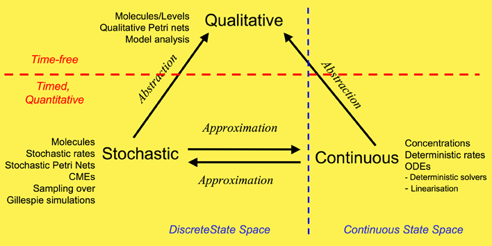
Our overall framework is illustrated in Figure 1 that relates the three major ways of modelling and analysing biochemical networks that we have used: qualitative, stochastic and continuous.
The most abstract representation of a biochemical network is qualitative and is minimally described by its topology. Initial descriptions can be obtained from biochemists, and are often in some semiformal representation. These can easily be transformed into a formal description at this stage which is usually a bipartite directed graph with nodes representing biochemical entities or reactions, or in Petri net terminology places and transitions (see Petri net section).
The qualitative description can be further enhanced by the abstract representation of discrete quantities of species, achieved in Petri nets by the use of tokens at places. These can represent the number of molecules, or the level of concentration, of a species. A particular arrangement of tokens over a network is called a marking. The standard semantics for these qualitative Petri nets (QPN) does not associate a time with transitions or the sojourn of tokens at places, and thus these descriptions are time-free. The qualitative analysis considers however all possible behaviour of the system under any timing. The behaviour of such a net forms a discrete state space.
Timed information can be added to the qualitative description in two ways -- stochastic and continuous. The continuous model replaces the discrete values of species with continuous values, and hence is not able to describe the behaviour of species at the level of individual molecules, but only the overall behaviour via concentrations. We can regard the discrete description of concentration levels as abstracting over the continuous description of concentrations. Timed information is introduced by the association of a particular deterministic rate information with each transition, permitting the continuous model to be represented as a set of ordinary differential equations (ODEs) (see Model Evolution). The concentration of a particular species in such a model will have the same value at each point of time for repeated experiments. The state space of such models is continuous and linear. It is also possible to linearise ODE descriptions, by for example Laplace transforms, in an attempt to increase modularity in the system description and hence to facilitate model construction (BioBrick library). This approach results in transformations from the time-domain, in which inputs and outputs are functions of time, to the frequency-domain.
The stochastic Petri net (SPN) description preserves the discrete state description, but in addition associates a probabilistically distributed firing rate or rate constant (waiting time) with each reaction and an associated rate law or hazard function which depends on the state of the system. Thus, the time-evolution of a reaction can be regarded as a stochastic process, and the time-evolution of the states of such a reaction system can be regarded as a Markov process with a discrete state space. In this context we can refer to the Chemical Master Equation (CME), which is equivalent to Kolmorogov's forward equation for a stochastic kinetic process (Wilkinson, 2006). It is quite straightforward to simulate such a system, and this is usually done with the standard discrete event simulation procedure known as "the Gillespie algorithm" (Gillespie, 1977). In our project we have directly simulated the system from CMEs using the Gillespie algorithm (Stochastic Modelling). The QPN is an abstraction of the SPN, sharing the same state space and transition relation with the stochastic model, with the probabilistic information removed. All qualitative properties valid in the QPN are also valid in the SPN, and vice versa.
In summary, the qualitative
time-free description is the most basic, with discrete values
representing numbers of molecules or levels of concentrations.
The qualitative description abstracts over two timed, quantitative models.
In the stochastic description, discrete values for the amounts of species
are retained, but a stochastic rate is associated with each reaction. The continuous model describes amounts of species using continuous values
and associates a deterministic rate with each reaction.
These two time-dependent models can be mutually approximated by hazard
functions belonging to the stochastic world.
Model Development
Sed ut perspiciatis unde omnis iste natus error sit voluptatem accusantium doloremque laudantium, totam rem aperiam, eaque ipsa quae ab illo inventore veritatis et quasi architecto beatae vitae dicta sunt explicabo. Nemo enim ipsam voluptatem quia voluptas sit aspernatur aut odit aut fugit, sed quia consequuntur magni dolores eos qui ratione voluptatem sequi nesciunt. Neque porro quisquam est, qui dolorem ipsum quia dolor sit amet, consectetur, adipisci velit, sed quia non numquam eius modi tempora incidunt ut labore et dolore magnam aliquam quaerat voluptatem. Ut enim ad minima veniam, quis nostrum exercitationem ullam corporis suscipit laboriosam, nisi ut aliquid ex ea commodi consequatur? Quis autem vel eum iure reprehenderit qui in ea voluptate velit esse quam nihil molestiae consequatur, vel illum qui dolorem eum fugiat quo voluptas nulla pariatur?
Parameter searching
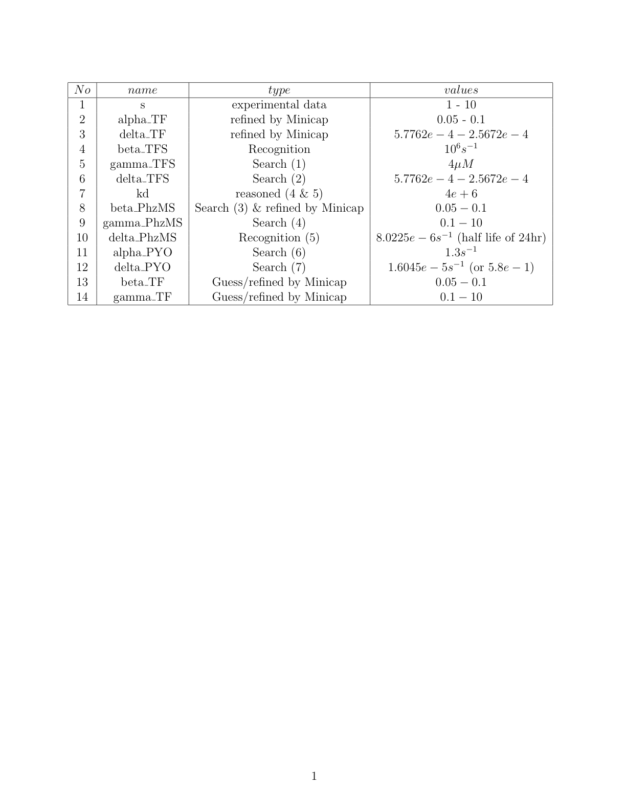
Parameter searching using Google Scholar, PubMed and biomedical databases was carried out by Christine and Xu under the direction of Dr David Leader. The task was largely steered by the discussions with, and the suggestions given by Emma Travis. We applied the Minicap program, developed as part of the project, in order to help us identify sensible ranges associated with the parameters. A complete table containing either exact or constrained values for each of the system parameters was produced, as shown in the [Parameters.png parameter table], where parameters are annotated with their type, values and supporting data sources.
Stochastic Modelling
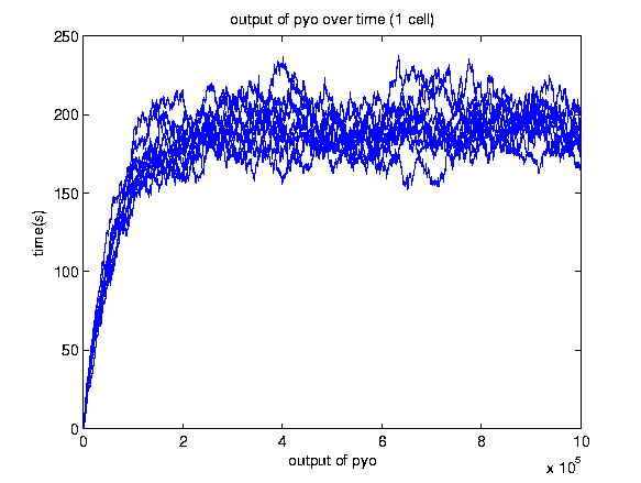
A stochastic model for a general biosensor was constructed by students and simulated using Gillespie algorithm in MATLAB. Modelling biological systems in terms of ordinary differential equations is often not enough as cells are intrinsically noisy due to low numbers of molecules that participate in reactions. This can lead to significant statistical fluctuations in reaction rates and systems behaviour can differ from the one predicted by a deterministic model. In this case, the system of interest was a single cell or bacteria of a bacterial whole cell biosensor.
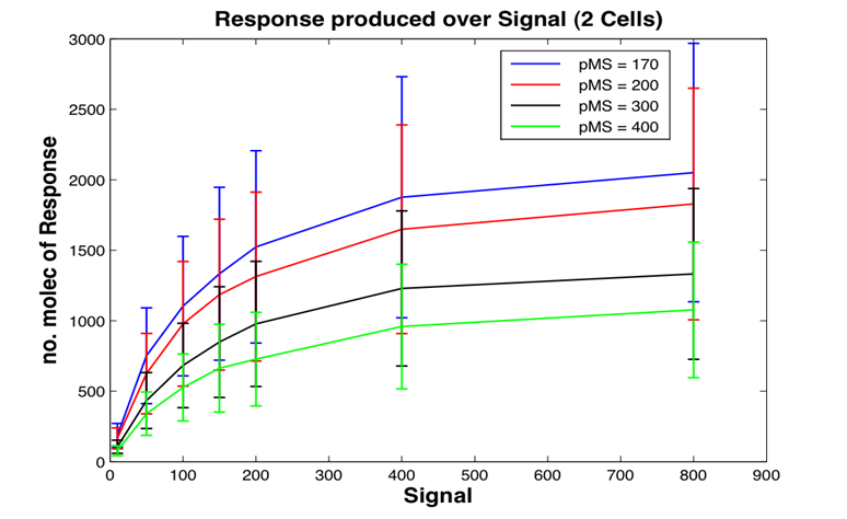
In this study the concept of stochastic simulation was introduced using a computational approach called Gillespie algorithm. The Gillespie algorithm allows a discrete and stochastic simulation with few reactants because every reaction is individually simulated. It takes into account a number of parameters that contribute to the model in a random manner, rather than assuming everything can be predicted. The goal of this study was to construct a stochastic model based on a deterministic one and to investigate the amount of noise (measured by the Fano factor and the coefficient of variation). Simulations were performed for several of cells and repeated for many runs to find representative behaviour. Noise was expected to decrease as the number of cells increased. However, in this study it was found that the coefficient of variation stayed roughly the same as the number of cells increased.
We also aimed to study whether generic features predicted by other modelling approaches can be repeated by stochastic simulations. The effects of leakiness of the promoter and positive feedback were also observed in the system. Leakiness had a detrimental effect on the reliability of the system. It provides a higher output of the protein which in turn gives a false indication of the level of signal being detected. Positive feedback gives a higher output of the protein but the system is significantly more noisy.
Full report on stochastic modelling
Model Analysis
Sed ut perspiciatis unde omnis iste natus error sit voluptatem accusantium doloremque laudantium, totam rem aperiam, eaque ipsa quae ab illo inventore veritatis et quasi architecto beatae vitae dicta sunt explicabo. Nemo enim ipsam voluptatem quia voluptas sit aspernatur aut odit aut fugit, sed quia consequuntur magni dolores eos qui ratione voluptatem sequi nesciunt. Neque porro quisquam est, qui dolorem ipsum quia dolor sit amet, consectetur, adipisci velit, sed quia non numquam eius modi tempora incidunt ut labore et dolore magnam aliquam quaerat voluptatem. Ut enim ad minima veniam, quis nostrum exercitationem ullam corporis suscipit laboriosam, nisi ut aliquid ex ea commodi consequatur? Quis autem vel eum iure reprehenderit qui in ea voluptate velit esse quam nihil molestiae consequatur, vel illum qui dolorem eum fugiat quo voluptas nulla pariatur?
Petri Net Modelling
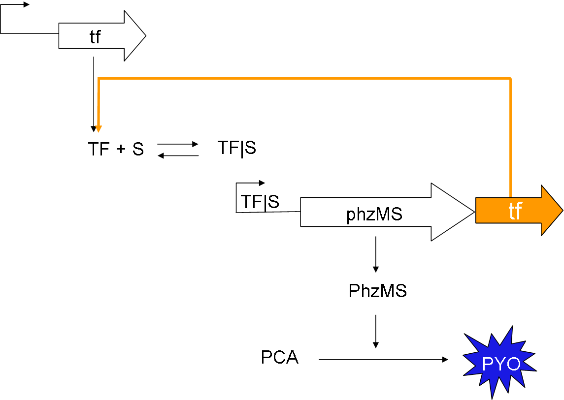
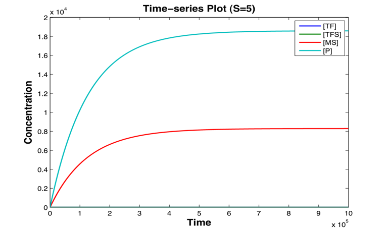
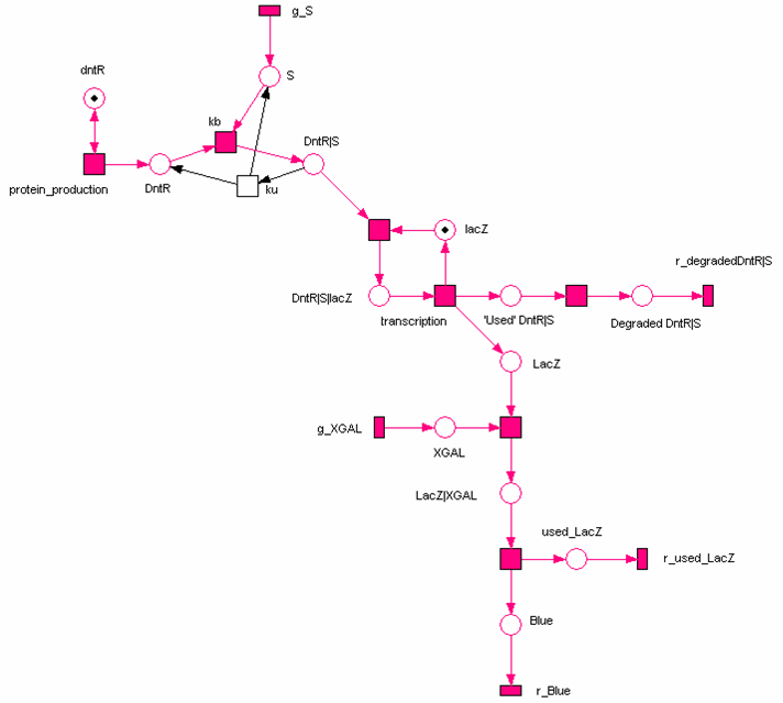
[http://en.wikipedia.org/wiki/Petri_nets Petri nets] are used to describe discrete distributed systems that have concurrent processes, and provide users with an intuitive and easy-to-understand graphical representation of systems. During the iGEM project, we explored the use of Petri nets for the construction and analysis of synthetic biological networks, with a focus on facilitating the experimental design. We started off with the construction of qualitative petri-net models using the [http://www-dssz.informatik.tu-cottbus.de/index.html?/software/snoopy.html Snoopy] tool. A major advantage of the Qualitative Petri net (QPN) approach is that it enables us to perform network analysis in the absence of prior knowledge of the system parameters. We achieved this using the Charlie tool (available from [http://www-dssz.informatik.tu-cottbus.de/index.html?/software/tutorial_biopn.html Monika Heiner], where we identified the subsets of the Petri net models covered by certain properties with T-invariants (cyclic behaviour) and P-invariants (constant output in amount). We also studied various suggestions for the system's possible structures using the token game with different initial markings. Based on the observation of possible flows and discussions with biochemists, we examined and validated the models in terms of the boundedness, for example. Although Petri Nets were initially designed for qualitative analysis they have been extended to permit other forms of analysis including the quantitative form which is known as a Continuous Petri Net (CPN) which has an ODE-based semantics (see framework). We investigated the dynamics of the systems quantitatively using the parameters retrieved from the literature (for details, please refer to the section on Parameter Searching), and simulated the behaviour using Snoopy's inbuilt ODE solvers. These results were consistent with those generated by the pure ODE approach.
Minicap Sensitivity Analysis Program Package
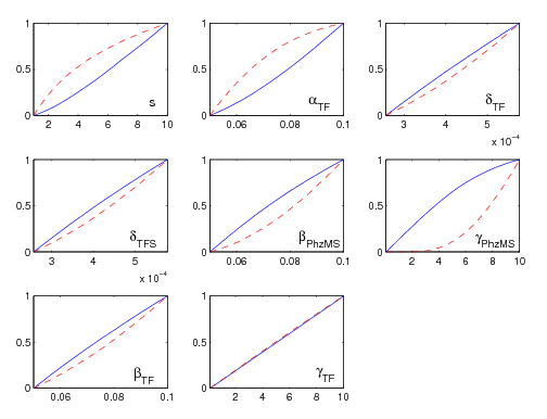
The Multi-Parametric and Initial Concentration Sensitivity analysis [http://compbio.dcs.gla.ac.uk/iGEM2007/Minicap_Sensitivity_Analysis_Program_Package.zip server (Minicap)] package is a Matlab function which executes a chosen Dynamic or Stochastic System Function for a defined number of different variable values across any desired range. The subject of analysis can either be constants in the user's system eg. parameters in a biological system (MPSA) or initial values of the variables in the user's system eg. initial substrate concentrations (ISCSA). The program will output a plot for each variable showing a comparison of acceptable and unacceptable samples across the subject's range with 3 calculated quantitative comparison figures: the Correlation Coefficient, the Area between acceptable and unacceptable curves, and the Standard Deviation of the gradient of the acceptable plot. The comparative and intrinsic sensitivity of each chosen subject is thus highlighted. A plot showing the trend of the Substrate of Interest over time is also displayed.
As well as this report, the Minicap package contains a User Manual in html, a number of example codes and all the novel (i.e. not ode15s) function and text files required to run Minicap.
To see the full PDF report on Minicap [click here].
BioBrick library
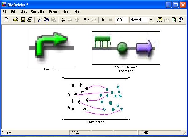
[http://compbio.dcs.gla.ac.uk/iGEM2007/BioBricklibrary.zip BioBrickLibrary.zip] An add on Library to Simulink for modelling dynamical biological systems at Brick (Gene) level. Simulink is a program dedicated for dynamical system simulation, however in depth knowledge of dynamics is needed if one is to simulate system mentioned above. The BioBrick library has all the blocks as well as GUI (Graphical User Interface) needed to do the job without understanding how Simulink works. It uses drag and drop system and shares all constants in Matlab’s .m file, so it is easy to store and update them.
BioBrick library’s main aim is to tell whether and how different topology will influence the output of the system. If actual rate constants are known it can be used instead or as complimentary to ODE modelling. However it must be noted that ODE rate constants ARE NOT TRANSFERABLE to BioBrick library.
More information can be found in ElectrEcoBluSimulinkManual document. See full Technical Report (BioBrick Type Modeling) for concept evolution and justification.
Microbial Fuel Cell Evaluation
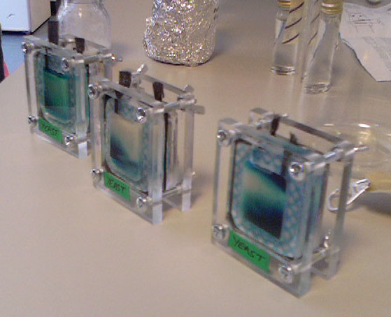
During the course of the project some introductory work has been done with microbial fuel cells in order to prepare us for the envisaged final stage of the project. We have had three fuel cells at our disposition supplied by the UK's NCBE. The experience we have gained and some of the results have been aggregated in this short work.
| Modelling | Log | Tutorials | References |
