Edinburgh/DivisionPopper/Modelling
From 2007.igem.org
Luca.Gerosa (Talk | contribs) (→ODEs (deterministic and continuous)) |
Luca.Gerosa (Talk | contribs) |
||
| Line 268: | Line 268: | ||
==== PoPS signal ==== | ==== PoPS signal ==== | ||
| + | |||
| + | {| border="1" cellpadding="20" cellspacing="0" | ||
| + | !Phase | ||
| + | !Equations | ||
| + | |- | ||
| + | |Forward Phase: | ||
| + | |||
| + | [[Image:proofforwardprocesses.png|600px]] | ||
| + | | | ||
| + | |- | ||
| + | |Flipping Phase: | ||
| + | |||
| + | [[Image:proofflippingprocesses.png|600px]] | ||
| + | | | ||
| + | |- | ||
| + | |Backward Phase: | ||
| + | |||
| + | [[Image:proofbackwardprocesses.png|600px]] | ||
| + | | | ||
| + | |- | ||
| + | |} | ||
| + | |||
====Results==== | ====Results==== | ||
Revision as of 17:21, 1 October 2007
MENU : Introduction | Background | Applications | Design&Implementation | Modelling | Wet Lab | Synthetic Biology Approach | Conclusions
This pages contains the mathematical and computational models we constructed in order to analyze the behaviour of the Division PoPper system. You can find the model of two systems (the proof of concept construct and the whole construct), different views on the system (the single cell behaviour or the behaviour of the population), different approaches to modeling (ODEs, CTMC, hybrid). Look at the table of contents below for the section you are interested in.
Contents |
The proof of concept system
As explained in the design section, the first part of our project consists in the realization of a proof of concept system. This is a smaller and less complex construct that we use to test our main assumption: the DNA region in between the two Dif sites is "flipped" (reversed) at each cell division. The model should help us in answering the following questions:
- Is the system working well with standard E.Coli division time?
- Is the system working well with normal YFP, GFP Expression and degradation rate?
- How can we tune these parameters in order to have meaningful tests from the construct in the lab?
Since the mechanisms and the values that characterize the system are sometimes not known or time consuming/difficult to discovery in the lab, we use the models as "in silico" test. Thus our models should be dependent (functions of) on the following quantities:
- Cell division frequency (units: minutes): is the time elapsed from one division to the next one.
- Flipping duration (units: minutes): is the time elapsed from starting the flipping to the complete execution.
- YFP/GFP Expression rate (units: protein per second): the rate at which fluorescent proteins are expressed.
- YFP/GFP Degradation rate (units: protein per second): the rate at which fluorescent proteins degrade.
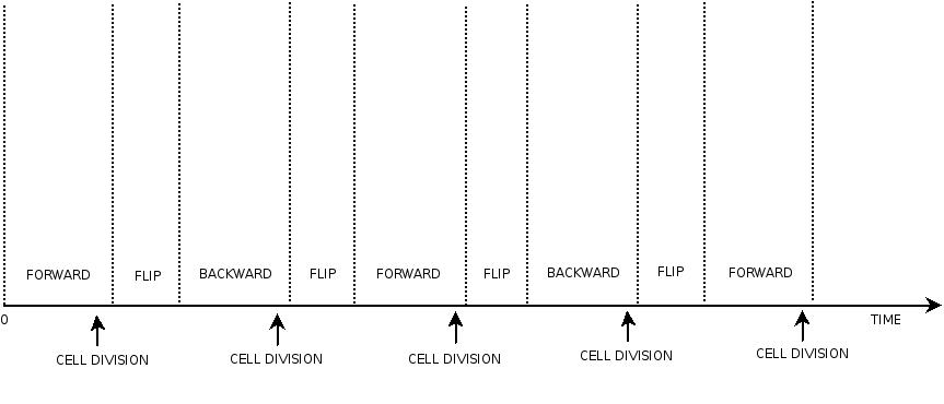
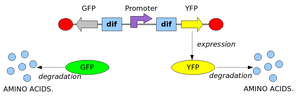
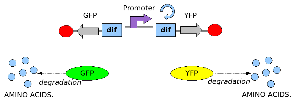
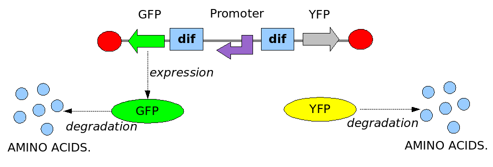
In order to construct the proper model, we need to identify which are the dynamics of the system. Since the real biological mechanisms are too complex, several approximations and abstractions are introduced at this step. In this sense, we can simplify the dynamics of the system by observing that three are the states in which our construct can be during the time evolution: Forward, Flipping and Backward phase. This three phases happen in a order controlled by cell division. In detail:
This three are the states (phases) in which the proof of concept system can be during its time course evolution. The system passes through these phases according to cell division timing and following the pattern: forward phase, flipping phase, backward phase, flipping phase and so on. A picture clarifies better the time course behaviour:
The arrows mark the points in time in which a cell division starts.
Modelling a single cell
As first step, we are interested in investigating the behaviour of the system at the level of a single cell. In particular, we are interested in following the course time behaviour of one single cell line. This means that in our model we start observing a individual cell behaviour and at each cell division we follow one of the two daughter cells and so on.
For that we construct two different approaches: using Ordinary Differential Equation and Stochastic Process Algebras. The first is deterministic (the behaviour of the system is defined only by the value of the variables) and treats population of molecules as a continuos value. It gives us a general understanding of what is the "avarage" behaviour of the time evolution of a cell. The second is stochastic (the behaviour of the systems is defined by the value of normal and random variables) and treats the population of molecules as a discrete value. It gives us (theoretically) a better understanding of which can be the different trajectory in behaviour of individual cells and helps us in simulating then the behaviour of a population.
ODEs (deterministic and continuous)
We define a set of ordinary differential equations that represents the behaviour of a individual cell during time. For first, we define a set of equations for each one of the three phases (Forward, Flipping, Backward) and then we construct a unified set of equations by using two support functions. The concentrations in which we are interested are obviously GFP and RFP concentrations. The biological mechanisms (or processes) we need to represent are: gene expression of proteins and degradation of proteins. We assume gene expression of a protein to be in on or off state and, when in the on state, to be expressed at a constant rate. We assume degradation of a protein to be rate dependent on the amount of protein present. Thus the variables are:
- YFP expression rate (mol/sec) called YFPexp
- GFP expression rate (mol/sec) called GFPexp
- YFP degradation rate (1/sec) called YFPdeg
- GFP degradation rate (1/sec) called GFPdeg
For each phase the set of equations are:
| Phase | Equations |
|---|---|
| Forward Phase: | d[YFP]/dt = YFPexp - YFPdeg*[YFP]
d[GFP]/dt = - GFPdeg*[GFP] |
| Flipping Phase: | d[YFP]/dt = - YFPdeg*[YFP]
d[GFP]/dt = - GFPdeg*[GFP] |
| Backward Phase: | d[YFP]/dt = - YFPdeg*[YFP]
d[GFP]/dt = GFPexp - GFPdeg*[GFP] |
In order to construct a model that represents the sequence of phases we introduce two support functions called respectively ForwardPhase(t) and BackwardPhase(t). They are time depending: ForwardPhase(t) returns value 1 when the system is in the Forward phase and 0 elsewhere, BackwardPhase(t) returns value 1 when the system is in the Backward Phase and 0 elsewhere.
Then the whole system is defined by equations:
d[YFP]/dt = YFPexp*ForwardPhase(t) - YFPdeg*[YFP]
d[GFP]/dt = GFPexp*BackwardPhase(t) - GFPdeg*[GFP]
The data for the expression and degradation rates and the have been taken from peer-reviewed publications as reference values and summarized in the table below:
| Data | Values | Reference |
|---|---|---|
| YFP expression rate | ||
| GFP expression rate | ||
| YFP degradation | ||
| GFP degradation | ||
| Flipping duration | ||
| Expression duration |
We implemented this model using the [http://www.sbtoolbox.org/ Systems Biology Toolbox for MATLAB] and the related code can be downloaded here.
The graphs representing the system behaviour are coming soon.
CTMC (stochastic and discrete)
Obviously the behaviour simulated by the ODEs system accounts as an "average" behaviour: we do not expect all cells to be exactly in the same state during time. Moreover we know that physically populations are not continues values but change in a discrete way. In order to deal with the implicit stochasticity and diversity of biological system, in the last years stochastic approaches have been investigated. In our case we use an approach based on [http://en.wikipedia.org/wiki/Process_calculi Process Algebras] (as formalism to define the system) and [http://en.wikipedia.org/wiki/CTMC Continuos Time Markov Chain (CTMC)] (as mathematical model). The Process Algebra we use to define the system is [http://www.dcs.ed.ac.uk/pepa/ PEPA], developed in Edinburgh University. For each specie, we define a set of PEPA processes, each one representing a possible population level. Then we add some stochastic actions representing the event of expressing a protein or degrading a protein. The PEPA definitions are:
YFP(I)= (YFPexp,rYFPexp).YFP(I+1) + (YFPdeg,rYFPdeg).YFP(I-1)
for 0<I<maxYFP, where maxYFP is the maximal number of molecules of YFP
GFP(I)= (GFPexp,rGFPexp).GFP(I+1) + (GFPdeg,rGFPdeg).GFP(I-1)
for 0<J<maxGFP, where maxGFP is the maximal number of molecules of GFP
FORWARDPHASE= (YFPexp,rYFPexp).FORWARDPHASE + (ChangePhaseToFlipping,rChangePhaseToFlipping).FLIPPINGPHASE1
FLIPPINGPHASE1= (ChangePhaseToBacward,rChangePhaseToBacward).BACKWARDPHASE
FLIPPINGPHASE2= (ChangePhaseToForward,rChangePhaseToForward).FORDWARDPHASE
BACKWARDPHASE= (GFPexp,rGFPexp).BACKWARDPHASE + (ChangePhaseToFlipping,rChangePhaseToFlipping).FLIPPINGPHASE2
The exponential rates are:
| Data | Values | Reference |
|---|---|---|
| rYFPexp | ||
| rYFPdeg | ||
| rGFPexp | ||
| rGFPdeg | ||
| rChangePhaseToFlipping | ||
| rChangePhaseToForward | ||
| rChangePhaseToBacward |
The system initial configuration is then:
YFP(initYFP)<YFPexp>FORWARDPHASE<GFPexp>GFP(initGFP)
where initYFP is the initial number of YFP molecules and initiGFP is the initial number of GFP molecules
Using CTMC we are forced to use a stochastic event also for division time. We assume the division time and the flipping time to be exponential distributed. From the initial configuration is possible then to derive the underlying CTMC of the model. Because of the simplicity of the system, we have implemented it directly in [http://www.prismmodelchecker.org/ PRISM] (the code can be downloaded here) and then simulated the CTMC (using the [http://en.wikipedia.org/wiki/Gillespie_algorithm Gillespie Algorithm]). A single simulation looks like:
(coming soon)
NB:
This approach can be used to model more complex systems (pathways and gene networks for examples). A graphical notation used as human interface to process algebra, the theoretical background, guidelines and case studies of this approach are the Master Dissertation topic of one of the team member (Luca Gerosa). The document will be uploaded after graduation (December 2007).
Results
Modelling a population
Coming soon
Hybrid (stochastic/deterministic and discrete)
Results
The Division PoPper device
Modelling a single cell
We replicate the same approach used in the Proof of Concept modelling. In this case the configuration of the construct in the different phases and the biological processes involved have been reported in detail in the Design section. The most important differences with the Proof of Concept model are the repression of the Tet and CLambda promoter by the transcriptional factors and the need to model the behaviour of the PoPS signal. The data for the expression and degradation rates and for modelling the repression processes have been taken from peer-reviewed publications as reference values and summarized in the table below:
| Data | Values | Reference |
|---|---|---|
| TetR repressor expression rate | ||
| CI lambda repressor expression rate | ||
| TetR repressor influence on TetR promoter | ||
| CI lambda repressor influence on Cl lambda promoter |
ODEs (deterministic and continuous)
The Division PoPper deterministic model has been constructed in two slightly different versions. The first simulates the behaviour of the device when a reporter protein coding region is placed downstream itself. This is a classical situation when we try to proper miseaure the PoPS signal and so is interesting to predict. The second is a model in which we proper represent the pure PoPS signal. The way to model a PoPS behaviour is not a classic of modelling literature, so we add fun in understanding which are the best assumption and equations to use.
With reporter protein
For both repressing systems (Tet and Clamba) we used the "classical approach" by using the Hill Equation in order to relate the velocity of protein expression with the repressor concentration in the cell. In order to present the equations we assume that a generic protein A has been placed downstream Tet and CLambda promoter. This are the two equations governing the velocity of expression donwstream the two promoters:
d[A]/dt= (VmaxA * K^n / ([TetR]^n + K^n)) – KADeg [A]
d[A]/dt= (VmaxA * K^n / ([ClambdaR]^n + K^n)) – KADeg [A]
PoPS signal
| Phase | Equations |
|---|---|
| Forward Phase: | |
| Flipping Phase: | |
| Backward Phase: |


