Paris/Continuous model
From 2007.igem.org
| Line 1: | Line 1: | ||
{{Template:Paris_menu_modeling}} | {{Template:Paris_menu_modeling}} | ||
| + | <br> | ||
=Well mixed population model = | =Well mixed population model = | ||
Revision as of 22:34, 23 October 2007
Contents |
Well mixed population model
We present here a theoretical approach based on population dynamics. We consider here the case of a well mixed, homogenous, culture of the SMB organism, i.e. there is no space in this analysis and we follow only the variation of the different cell lines concentrations in the culture volume.
Derivation of the model
Let the variables g, s and d describe respectively the concentrations of germinal and so- matic cells and the conentration of DAP, then we can write for our system :
Equation (1a) describes the growth of the germinal cell population in presence of sufficient DAP (interaction represented by the Michaelis-Menten function) ; the term proportional to α2 is the differentiation into somatic cells by recombination of the CRE/LOX box, and the last term proportional to α3 is the germinal cells’ death. Equation (1b) is the variation of the somatic cells’ population, with the term proportional to α4 for somatic cells’ death. The last line describes DAP production by the somatic cells, and includes a degradation term. In absence of any quantitative details on assimilation of DAP by germinal cells and response to DAP levels, n and k are are to be considered as arbirary phenomenological parameters. We take however in the following n = 1 neglecting potential saturation related non-linearities for high DAP concentrations. The value of k corresponds to the DAP concentration for half-maximal growth rate, and could set experimenntally. We simplify the previous system by assuming that the evolution of d is rapid compared to the cellular growth, so that at this time scale we can take d' = 0 and write d = s α5/ α6 . This gives the two-variable system :
Redefinition of parameters k → kα6 /α5 and α3 → α2 + α3 leads to the simpler writing :
Let us do some rewriting :
and by redefining the time and most of the parameters we get :
The fixed points are (g = 0, s = 0) and the solution of :
Analysis of stability
Fixed point at the origin
Let us linearise the system (5a) close to the origin. For small perturbations
around (g = 0, s = 0) (5a) is equivalent to :
We look for a solution of the form ![]() , with
, with ![]() an arbitrary vector. The values of λ are the eigenvalues of the matrix in (7) and can be obtain here straightforwardly by
the characteristic polynomial : λ1 = −b, λ2 = −1, with respectively the eigenvectors
an arbitrary vector. The values of λ are the eigenvalues of the matrix in (7) and can be obtain here straightforwardly by
the characteristic polynomial : λ1 = −b, λ2 = −1, with respectively the eigenvectors ![]() .
.
The two eigenvalues are always negative : the origin is therefore always an attractive fixed point. For too weak initial concentrations of the two cellular types, the system is always going to die out.
Second fixed point, out of the origin
Let (g0 := β s0 , s0 := k/(α−1) ) be the non trivial solution of (6a). We can simplify the (5a) by
dividing the two equations respectively by g0 et s0 and by taking as new variables G := g/g0
and S := s/s0:
and with μ := α−1 = α1/α2− 1 :
The fixed point is now (G0=1,S0=1). We linearise system (9a) around this point and look for a solution close to it. Take x := G−G0 and y := S−S0 , close to (G0,S0) we can write by keeping only the first order terme of (9a) :
Looking for a solution of the form ![]() , we need to find the eigenvalues of the matrix in
(10). Solving the characteristic polynomial gives :
, we need to find the eigenvalues of the matrix in
(10). Solving the characteristic polynomial gives :
In order to determine the stability of the fixed point, let us examine the signs of the eigenvalues : λ1 is always negative, while λ2 is positive if μ/1+μ > 0. That is, by returning to the original parameters of (1) if α1 > α2 (more growth than recombination). In this case (which is expected) the fixed point (G0, S0) is unstable and the populations of the two cell lines diverge.
Conclusion
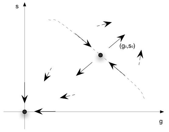
If we put together the results on the two fixed points we get the situation represented on the following diagram :

For a region around the origin and below some line passing through (G0, S0) any initial conditions converges to the origin. For higher values of the initial coonditions we always expect exponential growth of the populations.


