Davidson Missouri W/Mathematical Modeling
From 2007.igem.org
Contents |
Markov Chain Model For Flipping
Before spending time and resources in the wet lab, we wanted to model the biological systems in silico to better our understanding. A relatively simple, yet powerful, mathematical method is the use of Markov chains.
Does starting orientation matter?
Question: Will the initial order in which we place the edges in our E.coli computers affect the probability of us detecting a Hamiltonian Path?
Our mathematical reasoning relies on the fact that the Hin/hixC DNA recombination system makes a large number of flips and for any one flip there is some element of chance that dictates which hixC sites are chosen to flip.
Answer: We developed a Markov Chain model in Matlab that takes every signed permutation of edges as a state. Matlab then finds the connections between these states and categorizes them using both the number of edges that need to be flipped to move between those states, and which specific edges needed to be flipped. Further, our Matlab program creates a transition matrix based on user-inputted weights to bias the probabilities of making flips of varying sizes.
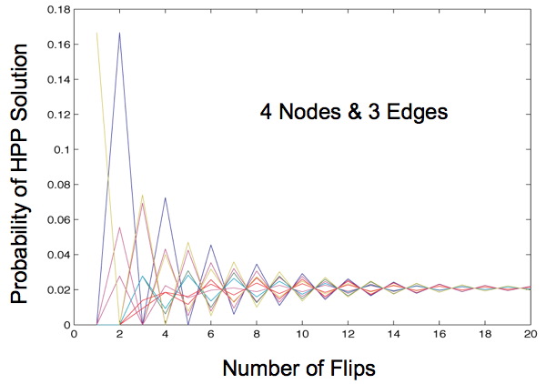
Once this transition matrix is generated, we compute, for each possible starting state, the probability that the starting state will transition to any of the solved states after x flips, given the biasing of different types of flips. When our Markov Chain model is run for more than 2 edges we always observe a convergence of these probabilities, regardless of any initial bias. This shows that starting orientation does not matter, since the probability of being solved after a large number of flips is the same for each starting orientation.
This begs the question: what is a large number of flips? Mostly we observe that this convergence occurs in the first 20 flips for three edges, and only for extreme probabilities does this convergence occur after 60 flips. However, as the number of edges increases, we can expect this convergence to occur later. This does not appear to be a problem in vivo. Our flipping mechanism flips edges quickly, so quickly that its speed is hard to measure. Additionally, the diameter of our transition diagrams increases linearly with the number of edges, so there is no reason to believe that the number of flips to convergence would increase at more than a linear pace.
MATLAB programs that we developed using Markov Chains:
- [http://gcat.davidson.edu/iGEM07/For_Missouri_Western/fliplength.m Flip Length]
- [http://gcat.davidson.edu/iGEM07/For_Missouri_Western/pureflip.m Pure Flip]
- [http://gcat.davidson.edu/iGEM07/For_Missouri_Western/biasweighter.m Bias Weighter]
Poisson Model For the Number of Plasmids
How many E.coli computers?
Question: If a Hamiltonian Path exists in the graph, how many E.coli computers do we need to have working on the problem to be highly confident that at least k of our computers will find it?
Our mathematical reasoning relies on the fact that the Hin/hixC DNA recombination system makes a large number of flips, and for any one flip there is some element of chance that dictates which hixC sites are chosen to flip. Note: This has now been shown to be true, but it needs to be stated that our math relies on it.
If this is the case, then our E. coli computers will be equally likely to have flipped into each possible signed ordering of edges by the time we screen our results. For more details on this see the above section about starting orientations.
We can use a cumulative Poisson distribution to answer this question.
Poisson is an appropriate distribution to use since:
1) The number of plasmids finding a solved state is a discrete random variable. 2) The probability of a plasmid finding a solved state is known and constant after convergence. 3) The probability of a plasmid finding a solved state is independent of other plasmids finding solved states.
Answer: The Poisson distribution gives the probability of k occurrences when the expected number of occurrences is λ as (e^-λ)*(λ^k)/(k!). By taking 1 minus the sum of the Poisson probabilities from 0 to k-1 we get the cumulative probability of at least k occurrences.
For example, examine the Adleman graph. It has 14 edges and 7 nodes. This means that a Hamiltonian Path is represented in our plasmids by 6 edges in the proper order and orientation followed by 8 edges in any order and in any orientation.
Thus there are 8!*2^8 orderings that are true positives and 14!*2^14 possible orderings. The probability of any one plasmid holding a true positive is then 8!*2^8 / 14!*2^14. If we have m plasmids, λ= m*8!*2^8 / 14!*2^14.
If we want to know the probability of at least one true positive in m plasmids then k = 1, and the expression becomes 1-(e^-(m*8!*2^8/14!*2^14)), as the summand collapses to the case where k=0 and (λ^0)/(0!) then equals 1.
We can then solve for m depending on how confident we want to be. If we use m=1 billion plasmids, then we expect to find the Hamiltonian Path when one exists 99.92% of the time.
1 billion E. coli computers fit conveniently into 1 mL of culture.
Using this statistical method we made a chart showing the probability of finding true positives based on the number of plasmids for the Adleman graph.
Probability of at least k solutions on m plasmids for Adelman's 14-edge graph
| k=1 | 5 | 10 | 20 | |
|---|---|---|---|---|
| m = 10,000,000 | 0.0697 | 0 | 0 | 0 |
| 50,000,000 | 0.3032 | 0.00004 | 0 | 0 |
| 100,000,000 | 0.5145 | 0.0009 | 0 | 0 |
| 200,000,000 | 0.7643 | 0.0161 | 0.000003 | 0 |
| 500,000,000 | 0.973 | 0.2961 | 0.0041 | 0 |
| 1,000,000,000 | 0.9992 | 0.8466 | 0.1932 | 0.00007 |
 , where n equals the number of solutions and κ equals actual number of occurrences. λ is the expected number of occurrences, which equals
 ![]() .
.
m = number of plasmids, s = number of solved permutations of edges, p = number of permutations of edges.
True Positives and False Positives
The crux of our experimental design is the simplicity of detecting answers phenotypically. Unfortunately, there exists the possibility that a phenotypically-correct colony may have an incorrect genotype. Although it looks like it has computed a solution, in fact it has not; this is known as a false-positive. We estimated the ratio of false-positives to true positives using Matlab simulations for several graphs.
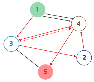
An example of a Hamiltonian Path in the above graph is shown with solid red arrows; below, its equivalent on a plasmid. There are in fact many possible true positive answers. Their PCR fragment lengths are identical, but the edges after the Hamiltonian path, following the transcriptional terminator node 5, can be arranged in any order. Some of these true positives might show the same path, whereas others may be different.
A false positive is represented in the graph above with the the dotted red arrow, which shows a "teleport". Teleporting occurs when an edge entering a node is followed by an edge leaving from a different node. Below you can see an extra edge that is highlighted, representing the teleport. In this example, the edge from 4 to 3 is followed by the edge from 4 to 5.
MATLAB programs used to find the false positives:
- [http://gcat.davidson.edu/iGEM07/For_Missouri_Western/fpVTgraph.m False positives for the 8 edge / 5 node graph shown above]. true positives = 384, false positives = 1,362
- [http://gcat.davidson.edu/iGEM07/For_Missouri_Western/davidson85Iweighter.m Counter Program for the 8 edge / 5 node graph]
- [http://gcat.davidson.edu/iGEM07/For_Missouri_Western/adelman147.m Adelman's false positives with 14 edges / 7 nodes]. true positives = 10,321,920, false positives = 168,006,848
- [http://gcat.davidson.edu/iGEM07/For_Missouri_Western/fpweighter.m Counter Program for Adelman's False Positives]
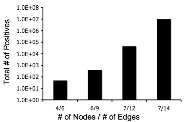
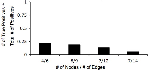
Below are two graphs that show how quickly the number of possible orderings of edges grows when the instance of the Hamiltonian Path Problem increases in the number of edges and nodes. This a Hamiltonian Paths harder to detect. Also, from these graphs you can tell that even though the graphs are becoming complex, there is still at least a 1 true positive for every 20 positives.


