Glasgow/Drylab
From 2007.igem.org
Contents |
Week 1
02/07
After a brief re-introduction to the Laboratory and our project proposal, we outlined a 6-PHASE approach to guide our practice over the summer.
From here the Modellers began working on basic Matlab modelling tutorials, designed by Xu Gu, to allow all modellers to reach a satisfactory ability. By the end of the day we had completed a number of Mass-action programs using the ode45 funtion and grasped the translation from basic notaion into Substrate, Enzyme and S/E-complex notation.
03/07
We developed our modelling techniques by programming responses to basic metabolic and signalling pathways. We then learnt more precise techniques of modelling, e.g. accuracy and tolerace variance and noting parameters. We then covered Loop and Switch functions.
04/07
We were introduced to the 'Nested Functions' to allow for simpler programming, and the basic ideas behind Sensitivity of output due to a range of possible values of varying constants.
In the afternoon, all modellers were shown some Wetlab techniques for the sake of a more thorough understanding of the processes involved.
Our experiment was to extract plasmids from a number of different bacterial cultures.
05/07
blank
06/07
Raya Khanin introduced us to the Michaelis-Menten equation and its use in biochemical process modelling. We then discussed the methods of modelling different promoters's 'Acceptablility', i.e. 'And', 'Or' and 'Sum'.
Week 2
09/07
Our first step towards modelling a possible method for PHASE 1.
10/07
We planned and gave a lecture to those in Wetlab, explaining the methods we employ, as modellers, to represent various biochemical reactions. We also received a complementary lecture from those in Wetlab explaining the processes they employ to carry out and observe experimentation.
11/07
We have finally agreed on model we are going to simulate, but wet lab updated us, that first experiment went wrong and we have to remodel. First few minutes after such news were shocking. It took us an hour to finalize all the details. And now we have to go again.
Lucky for us, modelers, computers dot care much about bacteria used in the experiment so as long as we follow the same pathway, we only need to rename variables. Bless!
12/07
A day dedicated to manual math's, as Rachel and Kristin does some analytical derivations for our model's optimization. To be honest, we were very optimistic about the outcome, and though, the formula derived were fine, and simulations went on as smoothly as ever, the optimization part shoved that 9 dimensional space is though nut to crack, even for MatLAB.
13/07
Some introduction to Stochastic Modelling intrinsicaly contained in gene transcription. We took some decisions about the design of the wiki. More optimization done by Maciej.
Week 3
16/07
Glasgow Bank Holiday.
17/07
We were given a brief introduction to Bionessie and SBML. Also we be begun to get to grips with Global Sensitivity analysis.
18/07
A brief overview of SimBiology was given to the drylab by Gary. Martina and Rachel continued learning about Stochastic modelling, while the rest of the team were working on Sensitivity Analysis.
19/07
A presentation was given to both, the wetlab and the drylab, about the Full Text Fetcher programme which, will help to search and retrive research articles. The Stochastic Simulation Algorithm (Gillespie's algorithm) is yet ready in the code to run some stochastics simulations on the Michaelis_Menten system.
20/07
Today we realized that, we missed few important details in our model 1. All morning was like one big mess. Everybody gave their ideas how things should be sorted. Eventually, we settled our brainstormed ideas on board and decided to leave simulations for Monday because new parameter hunt for model 1.2 was about to begin… Stochastic's work keeps on fitting the fano factor!
Week 4
23/07
Day spent on long discussions with Raya about the accuracy of our model 1.2 . We finally simulated it and… Results were a bit, shall I say, unpleasant. Because of signal degradation, we will not reach a stable state as we anticipated before. That is going to mess up our optimization algorithms, for sure.
24/07
Kristin was asked by Xu to introduce Petri Net([http://www-dssz.informatik.tu-cottbus.de/index.html?/~wwwdssz/software/snoopy.html Snoopy]) method to qualitatively analyse the dynamics of the system. And Karolis, introduced a dynamical approach in modeling of the system using Simulink. Both methods rely not only on blunt programming, but introduce GUI (Graphical User Interface) logics. Respect the Stochastic Model, we have been runing this one by doing some changes in the model (like changes in the signal, or other implementations), and later comparing with the deterministic model the results.
25/07
Maciek started a thorough research of registry files, because we were told by dry lab, that they are about to deposit their first brick and, it is not very intuitive (a good point for registry’s future development). He promised to study it and give us all tutorial about his findings. We have discussed as well about how we will determinate the parameters for the stochastic model.
26/07
Bricks. Brick Bricks. What is this brick? What is the aim of having bricks? All these questions were brought forward and we all agreed to do a thorough individual research and combine them in joint brainstorm, because as our grandfathers used to say: ‘There are as many opinions, as there are heads’. Reachel and Martina continue working in cascade models for Stochastics.
27/07
First bricks from Glasgow team reached a sandpit. No no. Do not rush to copy them. That’s just a ‘getting used to the system’. We are about to deposit real one, so we want everything to go as smooth as possible.
Week 5
30/07
Maciek’s tutorial enlightened wet and dry labs about all the registry’s pluses and minuses. We now know how to deposit a brick, edit it and etc. During this tutorial, we compiled a list of ides and suggestions, how to update the concept of brick itself, and some suggestions for registry’s future. Some questions have been asked by Rachael to the weblab to do some changes in the stochastic model.
31/07
To pursue the further ideas about Brick-Based system modeling Karolis introduced some CAD techniqes for possible GUI algorithm and code development. Rach, beautiful plots about the fano factor!! ;)
01/08
When the day was about to be over, we received long awaited news… First experimental data have finally reached us. We will be able to do some curve fitting, parameter estimation and other cool stuff?
02/08
Today we brainstormed the data we have. Everybody added their bit to ideas pot, however, since the data wasn’t that plentiful as we expected, we queried wet-lab for some more input. They promised, that more data is on the way. Stochastics are runing the code for several numbers of cells, and it take long time to run those!
03/08
Friday. The end of week 5. Our project just passed major milestone. No, not in development, but in time left available for us to complete it. We are, officially, halfway to successes now?
Week 6
06/08
Today we received extra data to support our estimations. General modelers meting raised issues like the further development of the model, feedback loops, or our possible influence for wet lab. Now, that we have some data, (input) we should produce some output for near future projects. Stochastics keep on runing simulations of data.
07/08
Day was full of events. First thing in the morning, we had a modelers meeting, to discuss our final model’s layout. General structure and equations were drafted on board. From now we will be analyzing previous data from lab and try to simulate new model, called Model F1.
Edinburgh team came to visit us after lunch. We exchanged some ideas about project, including modeling approaches and wet lab techniques used. After a brief introduction, we decided to continue our conversation outside the lab, so went to check what Glasgow could offer us.
08/08
Most of the day spent on Model F1, Model F1 Fedback and Model F1 Constitutive. Discussion about the stochastics full model to be able to compared with the deterministic one.
09/08
Even more types of models have been suggested to simulate. We have so much data now, so in order to manage it, we decided to document everything in LATEX. General standards are agreed for all the constants and equation. These are to be officially published later on. The propensities function reactions have been determinated for our stochastic model, let's go to codify them.
10/08
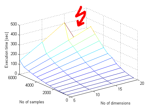
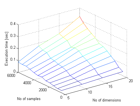
Today we realized, that even almighty MATLAB, is not always the best solution. Since our experiments require LHS (Latin Hypercube Sampling) in huge numbers and Matlab does it in one hour. We decided to switch back to Good Old C++. Job well done and in 10 SECONDS ONLY???!!!! What has just happened knows only Maciek himself. Only he knows The Way Of Gods.
Here I come to enlighten the oblivious. lhsdesign() in MATLAB is very slow for some reason. Moreover it seems to have polynomial complexity in number of samples while having linear complexity in number of dimensions.Why do we need so many samples anyway? Well, if you take 3 dimensional space and you take 1000 samples it will be only 10 samples along each axis! What if we want to have ONLY 10 samples along each axis in 21 dimensions? Well, we need 10e21 samples, oh!
A quick Google search leads to a mathematical library webpage at [http://www.scs.fsu.edu/ Florida State University] where a [http://people.scs.fsu.edu/~burkardt/cpp_src/latin_random/latin_random.html C++ code for generating samples from latin hypercube] is available. A big hand for them. We have tortured the latin_random_prb.C example file to create an interface and finally call it lhsdesign.c. It takes the number of samples and number of dimensions as command line arguments and writes the samples to standard output in a format that csvread likes. Inside MATLAB the file supadupalhsdesign.m provides the same interface as lhsdesign():
function samples = supadupalhsdesign(numsamples, numdimentions)
    system(['lhsdesign.exe ', num2str(numsamples),' ', num2str(numdimentions), ' > lhsout.csv']);
    samples = csvread('lhsout.csv');
end
What happens is the lhsdesign.exe is called using the system command and its output is directed into a temporary .csv file. Then the file is read into a matrix. Unfortunately we were not able to find a way to take the standard output of a command into a matrix directly, but it's not a major problem.
It's no rocket science, although Karolis says that rocket science is not so hard ;) Mcek
UPDATE 14/08: The C++ code for latin hypercube sampling wouldn't generate 200000 samples for 21 dimensions excusing itself with stack overflow. A look inside revealed that the array that stores the samples was static. A very quick
 double* x = NULL;
 x = new double[DIM_NUM*POINT_NUM];
...
 delete[] x;
 x = NULL;
fix was needed to allocate the array dynamically and our program is happy to give us 1 million samples in 23 dimensions and surely more! Mcek
Week 7
13/08
The day was quite productive, nerveless lucky. We manage to find 3 parameters of our interest. Besides that, we came with idea, how to compare qualitatively models F2 and F3 feedback. The method we developed and called ‘Feedback Logics’ allowed us to optimize four unknowns in F3 feedback. Results that came out suggested that addition of feedback loop for F3 will not influence the outcome of *** (sorry classified). Tomorrows meeting will decide, if F3 is wrong or it is the outcome one could expect.
14/08
All tests we were running today points that, we need to adjust our model ‘One Big F’, because model ‘F3 feedback; shows no influence for the final output. Wet lab said that they expect that ‘F3 feedback’ would change the repose in general. We have few, that still believe in parameter search, but their numbers are dwindling….
15/008
?
16/08
?
17/08
?

