Dry to Wet
From 2007.igem.org
(→Sensitivity) |
|||
| (40 intermediate revisions not shown) | |||
| Line 1: | Line 1: | ||
| - | === Mass-Action Reaction Modelling | + | {| valign=top cellpadding=3 |
| - | + | |- | |
| + | !align=center|[https://2007.igem.org/Glasgow https://static.igem.org/mediawiki/2007/thumb/c/cc/Uog.jpg/50px-Uog.jpg] || [[Glasgow|<font face=georgia color=#3366CC size=4>Back To <br> Glasgow's <br> Main Page</font>]] | ||
| + | |} | ||
| + | ---- | ||
| + | == Mass-Action Reaction Modelling == | ||
| + | There are many advantages of modeling a biological system in differential equations. Predictions can be made for experiments before they are carried out in the wetlab which can prove to be very useful. | ||
| - | [[Image: | + | The simplest reaction which is shown is simple decay where substance A decays to substance B. This can be modeled by two differential equations. The quantities which must be known to model these equations are the initial concentrations of both A and B and also the rate constant k1. By using Matlab a graph can be produced which shows that as A is used up B increases. |
| + | |||
| + | [[Image:simpledecayequation.jpg|400px]] | ||
| + | [[Image:simpledecay.jpg|400px]] | ||
| - | |||
| - | + | The decay reaction can also take the form of becoming a reversible reaction where A turns into B via a rate constant of k1 while at the same time B turns into A via a rate constant of k2. This again is modeled by two differential equations | |
| - | + | [[Image:reversibleequation.jpg|400px]] | |
| + | [[Image:reversible.jpg|400px]] | ||
| + | |||
| + | |||
| + | Another type of reaction which can be shown is an addition reaction where both A and B must be present to react to form C via a rate constant. Three differential equations are formed to model this reaction. | ||
| + | |||
| + | [[Image:additionequation.jpg|400px]] | ||
| + | [[Image:addition.jpg|400px]] | ||
| + | |||
| + | An enzyme reaction can be modeled as shown below. The enzyme complex is modeled by using both the addition reaction and the reversible reaction. | ||
| + | |||
| + | [[Image:enzymeequation.jpg|400px]] | ||
| + | [[Image:enzyme.jpg|400px]] | ||
| + | |||
| + | == RKIP network == | ||
After gaining a thorough understanding of methods involved with modeling simple mass-action reactions, we can move on to more complex systems such as the RKIP network.<br> | After gaining a thorough understanding of methods involved with modeling simple mass-action reactions, we can move on to more complex systems such as the RKIP network.<br> | ||
| - | [[Image:RKIP network.JPG]]<br> | + | [[Image:RKIP network.JPG | 700px]]<br> |
In the above diagram, substrates, enzymes and substrate/enzyme complexes are represented by numbered circles, rate constants are represented by numbered squares. By isolating individual species and their direct peripheral species (those being formed from or forming the isolated species) we are able to treat the group as a simple mass-action reaction. A differential equation is then found for each species based on the rate constants and code can be written and a graph plotted showing the trend of all the species’ concentration over time giving the following graph:<br> | In the above diagram, substrates, enzymes and substrate/enzyme complexes are represented by numbered circles, rate constants are represented by numbered squares. By isolating individual species and their direct peripheral species (those being formed from or forming the isolated species) we are able to treat the group as a simple mass-action reaction. A differential equation is then found for each species based on the rate constants and code can be written and a graph plotted showing the trend of all the species’ concentration over time giving the following graph:<br> | ||
[[Image:RKIP network graph.jpg]]<br> | [[Image:RKIP network graph.jpg]]<br> | ||
| - | + | == Sensitivity == | |
''An insight into a system's sensitivity will show how the variation of a model can be apportioned qualitatively or quantitatively to different sources of variation''<br> | ''An insight into a system's sensitivity will show how the variation of a model can be apportioned qualitatively or quantitatively to different sources of variation''<br> | ||
| - | One method of exposing the variation of a model is to program a loop exposing a modelled reaction to increasing values of a chosen constant. This process was followed with the metabolic pathway showing in | + | One method of exposing the variation of a model is to program a loop exposing a modelled reaction to increasing values of a chosen constant. This process was followed with the metabolic pathway showing in [[Mass-Action Reaction Modelling]] and ploted on a graph showing the response of all 4 species for a set range of varying K2 values from 1 to 10 where 10 is highlighted red.<br> |
| - | [[Image: metabolic sensetivity response]] | + | [[Image: metabolic sensetivity response.jpg | 800px]] |
| + | |||
| + | == Michaelis-Menten == | ||
| + | ''This was taken from 'Biochemistry' by 'Stryer'''<br> | ||
| + | ''I apologise for the format of the equations i did not have them in a pdf document and the mathematical formula toolbox will not work''<br><br> | ||
| + | Anybody who has done any sort of biological study will know Michaelis-Menten what i am trying to acheive here is to take it from the basics so as to equate it to the equations we will be using to model the system and to give the biologists an idea of what values and models we need. In this case all k values are rate constants and [] means concentration and E is enzyme, S is substrate and [E]t is total enzyme concentration. <br> | ||
| + | The Michaelis-Menten equation describes the kinetic properties of many enzymes. Consider the simple system A -> P | ||
| + | The rate of V is the quantity of A that disappears over a specified unit of time which is equal to the rate of appearance of P. For this system V=k[A] where k is the rate constant. | ||
| + | The simplest model that accounts for the kinetic properties of many enzymes is (i will add it in when i have figured out how to)<br> | ||
| + | what we want is an expression that relates the rate of catalysis to the concentrations of substrate and enzyme and the rates of the individual steps.<br> | ||
| + | Our starting point is that the catalytic rate is equal to the product of the ES complex and k3. | ||
| + | '''Vo=K2[ES]''' ''call this '''eqn(1)''' as i will be referring to it again'' | ||
| + | Now expressing [ES]in terms of known quantities the rates of '''formation''' and '''breakdown''' of [ES] are given by: | ||
| + | '''formation [ES] = k1*[E]*[S]''' | ||
| + | '''breakdown [ES] = (k2+k3)*[ES]''' | ||
| + | A steady state occurs when the rates of formation and breakdown of the ES complex are equal, this gives the formula | ||
| + | '''k1*[E]*[S]=(k2+k3)*[ES]''' | ||
| + | which then gives | ||
| + | '''[E][S] / [ES]=(k2+k3) / k1''' <br> | ||
| + | This can be simplified by defining '''Km''' called the Michaelis constant<br> | ||
| + | '''Km = (k2+k3) / k1''' | ||
| + | from this we get | ||
| + | '''[ES] = [E][S] / Km''' ''call this '''eqn(2)''' as i will be referring to it again'' <br> | ||
| + | Now examining the numerator of this equation: because substrate is usually present at much higher concentrations than the enzyme, the concentration of uncombined substrate [S]is very nearly equal to the total substrate concentration. The concentration of enzyme [E] is equal to '''[E]t - [ES]''' now substituting this into ''eqn(2)'' and after some simplification we get | ||
| + | '''[ES]=([E]t*[S]) / ([S]+Km)''' | ||
| + | by substituting this expression into ''eqn(1)'' we get | ||
| + | '''Vo = (k2[E]t*[S]) / ([s]+Km)''' | ||
| + | The maximised rate Vmax is obtained when the catalytic sites on the enzyme are saturated with substrate i.e '''[ES] = [E]t''' thus | ||
| + | '''Vmax = k2*[E]t | ||
| + | this gives the Michaelis-Menten equation | ||
| + | '''Vo = Vmax*([S] / ([S]+km)) ''' ''call this '''eqn(3)''' as i will refer to it again'' | ||
| + | when '''[S]=Km''' then '''Vo = Vmax / 2'''. Thus Km is equal to the substrate concentration at which the reaction rate is half its maximal value.<br> | ||
| + | |||
| + | ''The following part is from slides Raya showed us''<br> | ||
| + | Now relating this to gene transcription which we will be doing in this project. As any biologist will know<br> | ||
| + | '''Gene expression = production - degradation'''<br> | ||
| + | so '''μ’(t) = p(t) - δμ(t) ''' ''call this '''eqn(4)''' i will refer back to it''<br> | ||
| + | μ’(t) could be the production of mRNA for example. | ||
| + | '''where P(t) = production rate and δ(t) = linear degredation rate''' <br> | ||
| + | We have the Michaeilis Menton model for the production (or transcription) rate. There is one for the '''activator''' and one for the '''repressor'''.<br> | ||
| + | '''Activator'''- The transcription factor '''TF''' ''increases'' the transcription rate of the gene: | ||
| + | '''P(t)a =( β*[TF] / (γ + [TF]) ) + α''' ''call this '''eqn(5)'''''<br> | ||
| + | Where<br>β >0 is the maximum transcription rate which is equivalent to say '''Vmax''' in '''''eqn(3)'''''<br> | ||
| + | γ >0 is the half saturation constant which is equivalent to say '''Km''' in '''''eqn(3)'''''<br> | ||
| + | α >=0 is the basal rate of transcription (As far as i am aware this can be referred to as leakiness) which is taken into consideration to make the model more accurate.<br> | ||
| + | Now the equation for gene transcription for the '''activator''' is given by substituting '''''eqn(5)''''' into '''''eqn(4)''''' and assuming α=0. | ||
| + | '''μ’(t)a = ( β*[TF] / (γ + [TF]) ) - δμ(t) '''<br> | ||
| + | '''Repressor''- The transcription factor '''TF''' ''decreases''the transcription rate of the gene: | ||
| + | '''P(t)r =( β / (γ + [TF]) ) + α''' ''call this '''eqn(6)'''''<br> | ||
| + | Again the equation for gene transcription for the '''repressor''' is given by sunstituting '''''eqn(6)''''' into '''''eqn(5)''''' and assumingα=0. We get: | ||
| + | '''μ’(t)r = ( β / (γ + [TF]) ) - δμ(t) '''<br> | ||
| + | When considering more than one binding site we brinh '''h=number of binding sites into the equation''' so in both the '''activator''' and '''repressor''' equations for gene transcription '''whenever TF is in the equation you multiply it to the power of h'''. | ||
| + | |||
| + | == Multiple Transcription Factors == | ||
| + | |||
| + | There is an extension of the formulas from Michaelis-Menten, for '''multiple transcription factors'''. | ||
| + | |||
| + | ''Regulation of gene expression is controlled by the binding of transcription factors to specific DNA sequences in gene promoter regions. Multiple transcription factor binding events are involved in the regulation of cellular processes.'' | ||
| + | |||
| + | |||
| + | When we have more than one '''transcription factor''' (TF) involved we can find two situations:<br> | ||
| + | (In this page we will study the scenario with only 2 transcription factors involved) | ||
| + | |||
| + | - SUM Gate.<br> | ||
| + | - ADD Gate. | ||
| + | |||
| - | + | <u>'''SUM Gate'''</u>: As the word refers in this situation the effect from multiple TFs is additive. That means that the transcription could be induced for one '''OR''' other factor (or both together). But we have to note in this point that it’s not necessary the presence of both of them. | |
| - | + | <u>'''ADD Gate'''</u>: Implies the situation where the effect from multiple TFs is multiplicative. That means that the transcription will be induced for one '''AND''' the other factor at the same time (both actuate together). Nottice that if one of them is not active the transcription will not be done. | |
| - | == | + | <center>[[Image:formulas.jpg|400px]]</center> |
| + | == Modeling the behaviour in practice == | ||
Latest revision as of 13:48, 29 August 2007
| https://static.igem.org/mediawiki/2007/thumb/c/cc/Uog.jpg/50px-Uog.jpg | Back To Glasgow's Main Page |
|---|
Contents |
Mass-Action Reaction Modelling
There are many advantages of modeling a biological system in differential equations. Predictions can be made for experiments before they are carried out in the wetlab which can prove to be very useful.
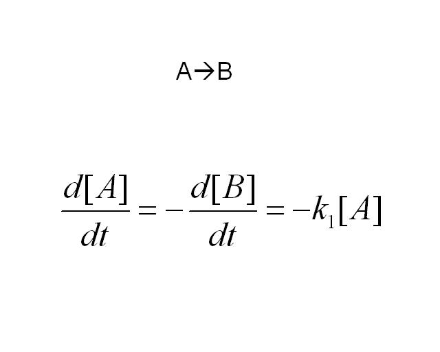
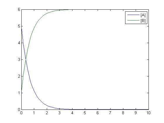
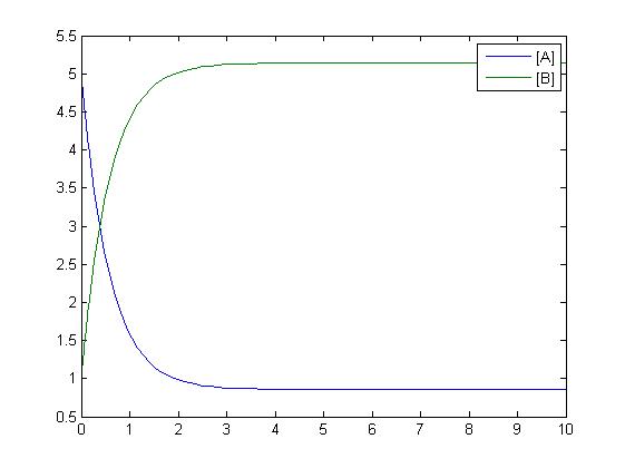
The simplest reaction which is shown is simple decay where substance A decays to substance B. This can be modeled by two differential equations. The quantities which must be known to model these equations are the initial concentrations of both A and B and also the rate constant k1. By using Matlab a graph can be produced which shows that as A is used up B increases.
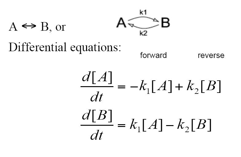
The decay reaction can also take the form of becoming a reversible reaction where A turns into B via a rate constant of k1 while at the same time B turns into A via a rate constant of k2. This again is modeled by two differential equations
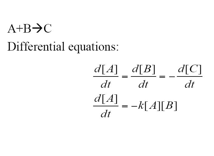
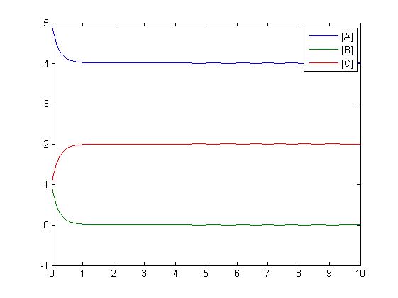
Another type of reaction which can be shown is an addition reaction where both A and B must be present to react to form C via a rate constant. Three differential equations are formed to model this reaction.
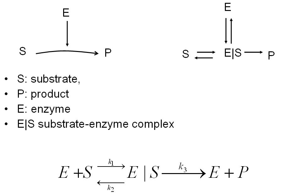
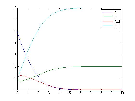
An enzyme reaction can be modeled as shown below. The enzyme complex is modeled by using both the addition reaction and the reversible reaction.
RKIP network
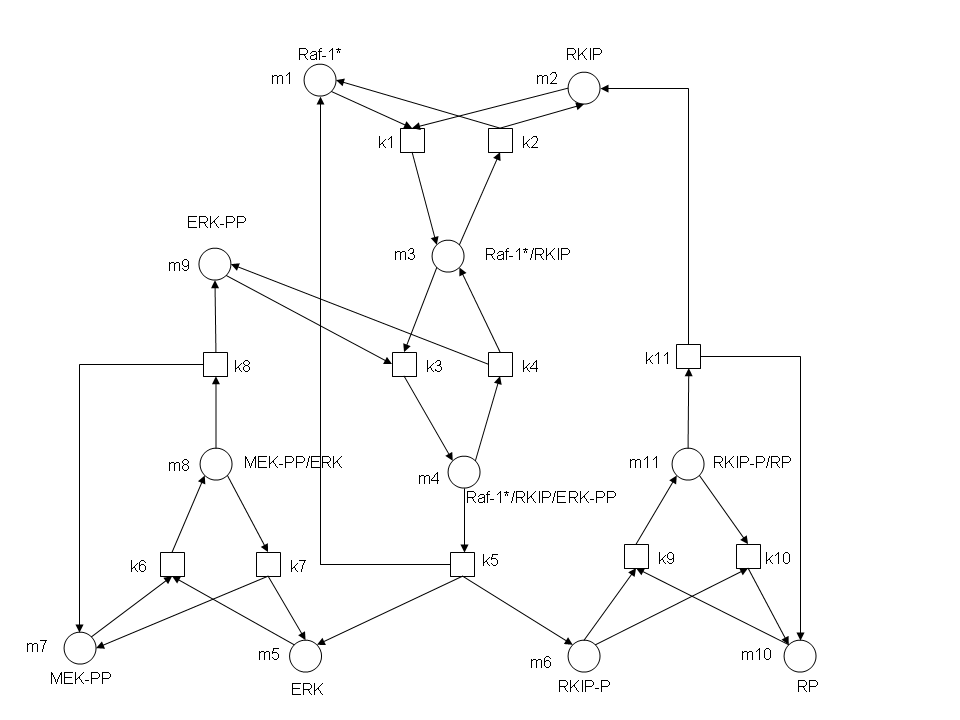
After gaining a thorough understanding of methods involved with modeling simple mass-action reactions, we can move on to more complex systems such as the RKIP network.
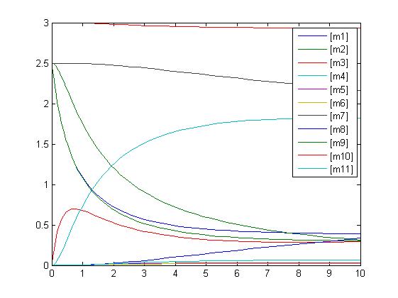
In the above diagram, substrates, enzymes and substrate/enzyme complexes are represented by numbered circles, rate constants are represented by numbered squares. By isolating individual species and their direct peripheral species (those being formed from or forming the isolated species) we are able to treat the group as a simple mass-action reaction. A differential equation is then found for each species based on the rate constants and code can be written and a graph plotted showing the trend of all the species’ concentration over time giving the following graph:
Sensitivity
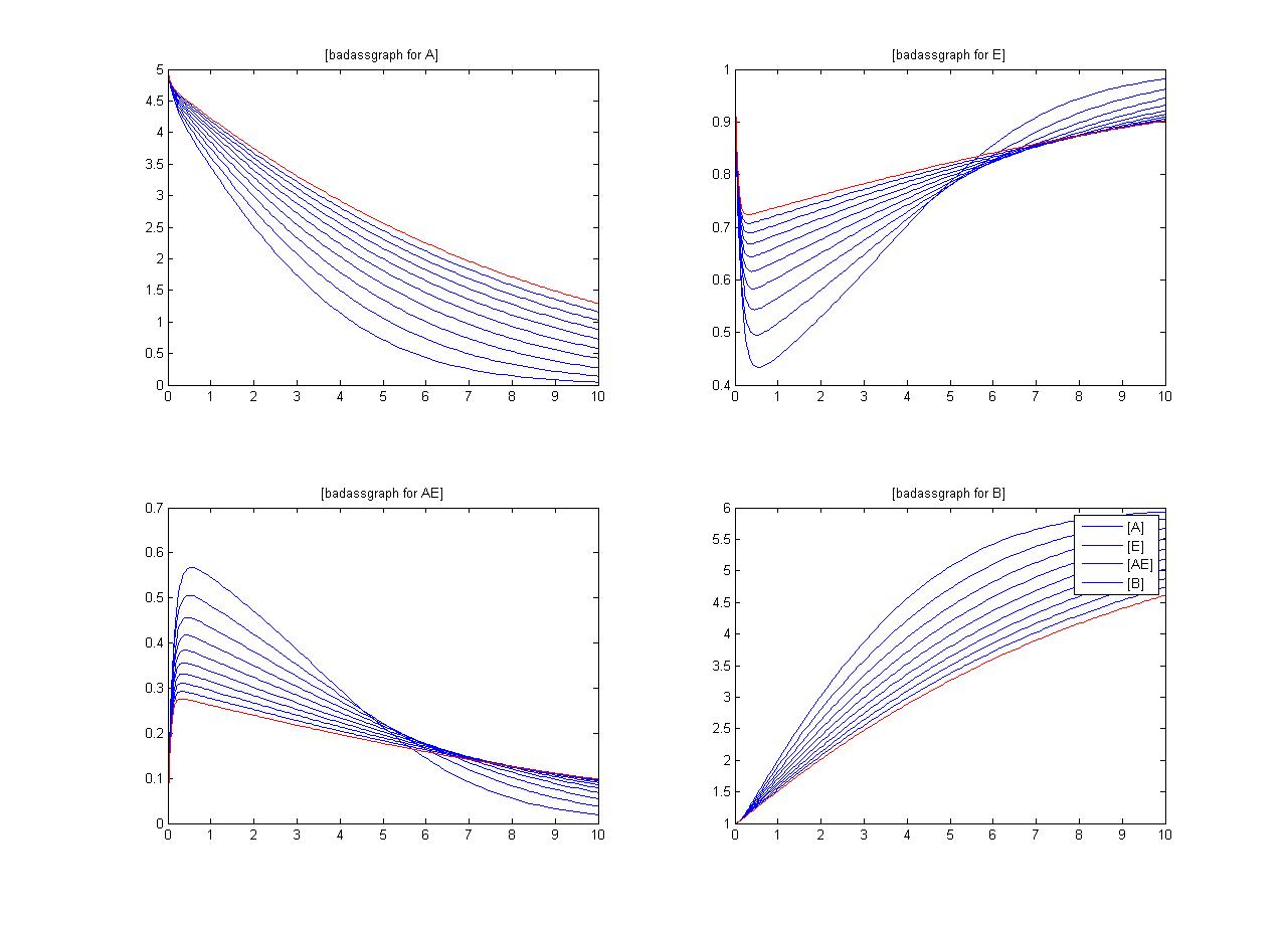
An insight into a system's sensitivity will show how the variation of a model can be apportioned qualitatively or quantitatively to different sources of variation
One method of exposing the variation of a model is to program a loop exposing a modelled reaction to increasing values of a chosen constant. This process was followed with the metabolic pathway showing in Mass-Action Reaction Modelling and ploted on a graph showing the response of all 4 species for a set range of varying K2 values from 1 to 10 where 10 is highlighted red.
Michaelis-Menten
This was taken from 'Biochemistry' by 'Stryer'
I apologise for the format of the equations i did not have them in a pdf document and the mathematical formula toolbox will not work
Anybody who has done any sort of biological study will know Michaelis-Menten what i am trying to acheive here is to take it from the basics so as to equate it to the equations we will be using to model the system and to give the biologists an idea of what values and models we need. In this case all k values are rate constants and [] means concentration and E is enzyme, S is substrate and [E]t is total enzyme concentration.
The Michaelis-Menten equation describes the kinetic properties of many enzymes. Consider the simple system A -> P
The rate of V is the quantity of A that disappears over a specified unit of time which is equal to the rate of appearance of P. For this system V=k[A] where k is the rate constant.
The simplest model that accounts for the kinetic properties of many enzymes is (i will add it in when i have figured out how to)
what we want is an expression that relates the rate of catalysis to the concentrations of substrate and enzyme and the rates of the individual steps.
Our starting point is that the catalytic rate is equal to the product of the ES complex and k3.
Vo=K2[ES] call this eqn(1) as i will be referring to it again
Now expressing [ES]in terms of known quantities the rates of formation and breakdown of [ES] are given by:
  formation [ES] = k1*[E]*[S]
  breakdown [ES] = (k2+k3)*[ES]
A steady state occurs when the rates of formation and breakdown of the ES complex are equal, this gives the formula
k1*[E]*[S]=(k2+k3)*[ES]
which then gives
[E][S] / [ES]=(k2+k3) / k1
This can be simplified by defining Km called the Michaelis constant
Km = (k2+k3) / k1
from this we get
[ES] = [E][S] / Km call this eqn(2) as i will be referring to it again
Now examining the numerator of this equation: because substrate is usually present at much higher concentrations than the enzyme, the concentration of uncombined substrate [S]is very nearly equal to the total substrate concentration. The concentration of enzyme [E] is equal to [E]t - [ES] now substituting this into eqn(2) and after some simplification we get
[ES]=([E]t*[S]) / ([S]+Km)
by substituting this expression into eqn(1) we get
Vo = (k2[E]t*[S]) / ([s]+Km)
The maximised rate Vmax is obtained when the catalytic sites on the enzyme are saturated with substrate i.e [ES] = [E]t thus
Vmax = k2*[E]t
this gives the Michaelis-Menten equation
Vo = Vmax*([S] / ([S]+km)) call this eqn(3) as i will refer to it again
when [S]=Km then Vo = Vmax / 2. Thus Km is equal to the substrate concentration at which the reaction rate is half its maximal value.
The following part is from slides Raya showed us
Now relating this to gene transcription which we will be doing in this project. As any biologist will know
Gene expression = production - degradation
so μ’(t) = p(t) - δμ(t) call this eqn(4) i will refer back to it
μ’(t) could be the production of mRNA for example.
where P(t) = production rate and δ(t) = linear degredation rate
We have the Michaeilis Menton model for the production (or transcription) rate. There is one for the activator and one for the repressor.
Activator- The transcription factor TF increases the transcription rate of the gene:
P(t)a =( β*[TF] / (γ + [TF]) ) + α call this eqn(5)
Where
β >0 is the maximum transcription rate which is equivalent to say Vmax in eqn(3)
γ >0 is the half saturation constant which is equivalent to say Km in eqn(3)
α >=0 is the basal rate of transcription (As far as i am aware this can be referred to as leakiness) which is taken into consideration to make the model more accurate.
Now the equation for gene transcription for the activator is given by substituting eqn(5) into eqn(4) and assuming α=0.
μ’(t)a = ( β*[TF] / (γ + [TF]) ) - δμ(t)
'Repressor- The transcription factor TF decreasesthe transcription rate of the gene:
P(t)r =( β / (γ + [TF]) ) + α call this eqn(6)
Again the equation for gene transcription for the repressor is given by sunstituting eqn(6) into eqn(5) and assumingα=0. We get:
μ’(t)r = ( β / (γ + [TF]) ) - δμ(t)
When considering more than one binding site we brinh h=number of binding sites into the equation so in both the activator and repressor equations for gene transcription whenever TF is in the equation you multiply it to the power of h.
Multiple Transcription Factors
There is an extension of the formulas from Michaelis-Menten, for multiple transcription factors.
Regulation of gene expression is controlled by the binding of transcription factors to specific DNA sequences in gene promoter regions. Multiple transcription factor binding events are involved in the regulation of cellular processes.
When we have more than one transcription factor (TF) involved we can find two situations:
(In this page we will study the scenario with only 2 transcription factors involved)
- SUM Gate.
- ADD Gate.
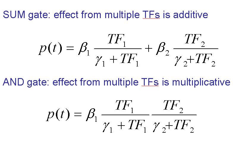
SUM Gate: As the word refers in this situation the effect from multiple TFs is additive. That means that the transcription could be induced for one OR other factor (or both together). But we have to note in this point that it’s not necessary the presence of both of them.
ADD Gate: Implies the situation where the effect from multiple TFs is multiplicative. That means that the transcription will be induced for one AND the other factor at the same time (both actuate together). Nottice that if one of them is not active the transcription will not be done.
