Saint Petersburg/Algebra
From 2007.igem.org
m (→Bistable behaviour of two repressors, mutually repressing each other) |
|||
| (6 intermediate revisions not shown) | |||
| Line 1: | Line 1: | ||
| - | + | ==Bistable behaviour of two repressors, mutually repressing each other== | |
| - | + | [[Saint_Petersburg|Main page]] | |
| + | |||
| + | [[Saint_Petersburg/ModelFormulation|Previous page - Model Formulation]] | ||
| + | |||
| + | ===Algebraic analysis of stabilty=== | ||
Graphical analysis and numeric modeling are obvious, but the algebraic solution is the most powerful for describing the modes of the behavior of the system, and finding optimal parameters. | Graphical analysis and numeric modeling are obvious, but the algebraic solution is the most powerful for describing the modes of the behavior of the system, and finding optimal parameters. | ||
| - | The system (III) may be reduced to one equation with one response variable: | + | The system [[Saint_Petersburg/ModelFormulation#Differential equations|(III)]] may be reduced to one equation with one response variable: |
| - | ''F'' (''X; P, Q, J, n, m'') = 0 | + | ''F'' (''X; P, Q, J, n, m'') = 0 (IVa) |
In our case the system will yield: | In our case the system will yield: | ||
| - | (IVb) | + | [[Image:spb_eqn_010.gif]] (IVb) |
If we solve this equation for ''X'', we will get all the stationary points for the system (III). Although the response ''X'' could be found only in few limited cases, stability analysis for our model could be performed in the most general case. | If we solve this equation for ''X'', we will get all the stationary points for the system (III). Although the response ''X'' could be found only in few limited cases, stability analysis for our model could be performed in the most general case. | ||
Fisrt we will find the bifurcation set. ''P'', ''Q'' and ''J'' form the ''control space'' of the system (''m'' and ''n'' are considered to be static parameters, as they are innate to the design and are not easily changed). ''Bifurcation set'' is the set of points in the control space, where the number of stationary points (system responses) change abruptly. That is the points where the roots of the equation (IV) has order higher than 1. In other words, bifurcation points are the points of discontinuity of partial derivatives ''dX/dp'' (''p'' - any parameter in ''F''). There is a well-known expression for parametric functions: | Fisrt we will find the bifurcation set. ''P'', ''Q'' and ''J'' form the ''control space'' of the system (''m'' and ''n'' are considered to be static parameters, as they are innate to the design and are not easily changed). ''Bifurcation set'' is the set of points in the control space, where the number of stationary points (system responses) change abruptly. That is the points where the roots of the equation (IV) has order higher than 1. In other words, bifurcation points are the points of discontinuity of partial derivatives ''dX/dp'' (''p'' - any parameter in ''F''). There is a well-known expression for parametric functions: | ||
| - | + | ||
| + | [[Image:spb_eqn_012.gif]] | ||
| + | |||
As our model is continious with respect to its parameters (linear with respect to ''P'', ''Q'', ''J'') a derivative ''dX/dp'' only becomes discontinuous when ''dF/dX'' = 0. So the bifurcation set is given by the system: | As our model is continious with respect to its parameters (linear with respect to ''P'', ''Q'', ''J'') a derivative ''dX/dp'' only becomes discontinuous when ''dF/dX'' = 0. So the bifurcation set is given by the system: | ||
| + | |||
| + | [[Image:spb_eqn_014.gif]] | ||
In our case the expression yields: | In our case the expression yields: | ||
| - | (V) | + | [[Image:spb_eqn_016.gif]] (V) |
In our case the system may be solved algebraically for the (''P'',''Q'') (''J'', ''P'') and (''J'', ''Q'') cross-sections. For the solution, that we omit for its clumsiness (thanks to math software), it is important that ''X'', ''P'', ''Q'' and ''J'' are significantly positive, and ''m'' and ''n'' are larger or equal to 1. It is required in several cases to state, that ''(Z<sup>1/N</sup>)<sup>N</sup> = Z''. The solutions are given in parametric form ''P''=''P''(''X''; ''J''), ''Q''=''Q''(''X''; ''J'') with ''X'' as a parametric variable. ''X'' may not be excluded in general case, but the cross sections of bifurcation set may be now plotted easily for any ''P'', ''Q'' and ''J''. | In our case the system may be solved algebraically for the (''P'',''Q'') (''J'', ''P'') and (''J'', ''Q'') cross-sections. For the solution, that we omit for its clumsiness (thanks to math software), it is important that ''X'', ''P'', ''Q'' and ''J'' are significantly positive, and ''m'' and ''n'' are larger or equal to 1. It is required in several cases to state, that ''(Z<sup>1/N</sup>)<sup>N</sup> = Z''. The solutions are given in parametric form ''P''=''P''(''X''; ''J''), ''Q''=''Q''(''X''; ''J'') with ''X'' as a parametric variable. ''X'' may not be excluded in general case, but the cross sections of bifurcation set may be now plotted easily for any ''P'', ''Q'' and ''J''. | ||
| - | + | ===The results=== | |
| + | |||
| + | Here we will discuss only the (''P'', ''Q'') cross section. In (''P'', ''Q'') cross section the bifuraction set is given by the following expression: | ||
| + | |||
| + | [[Image:spb_eqn_018.gif]] | ||
| + | |||
| + | To obtain the bifurcation curve here one should plot the second parameter versus the first, varying ''X'' from 0 to ''P+J''. The bifurcation curves for various m and n and no input signal provided are presented in Fig 2. | ||
| - | [[bifurc_PQ1.gif]] | + | [[Image:bifurc_PQ1.gif]] |
'''Figure 2. Bufurcation sets of cross-repressor system for various and equal cooperativity indices. The area of hysteretic behaviour for m=n=2 is filled with green.''' | '''Figure 2. Bufurcation sets of cross-repressor system for various and equal cooperativity indices. The area of hysteretic behaviour for m=n=2 is filled with green.''' | ||
| - | + | The two other cross sections could be viewed by following the links below: | |
| - | [[Saint_Petersburg/AlgebraJQ (J,Q)-cross section]]. Behaviour of the system at fixed efficiency ''P'' of the in-phase operator. | + | [[Saint_Petersburg/AlgebraJP|(''J'', ''P'')-cross section]]. Behaviour of the system at fixed efficiency ''Q'' of the out-of-phase operator. |
| + | |||
| + | [[Saint_Petersburg/AlgebraJQ|(''J'', ''Q'')-cross section]]. Behaviour of the system at fixed efficiency ''P'' of the in-phase operator. | ||
The bifurcation set has a typical ''cusp'' geometry. The two lines, leaving the cusp are the two ''fold catastrophes'' (they will be real folds if we visualize the response surface). In the region outside the cusp the system is monostable and the response is solely defined by the values of parameters (quasi-stationary). The system (III) has only one positive solution. Inside the cusp the system is bistable. Three roots for system (III) exist, one of them correspond to unstable saddle point – transition state. The dynamic system (II) has to have ''hysteresis'' – the responce will depend on the previous history of the process. The amplitude of hysteresis increase rapidly as we get deeper into the cusp region. | The bifurcation set has a typical ''cusp'' geometry. The two lines, leaving the cusp are the two ''fold catastrophes'' (they will be real folds if we visualize the response surface). In the region outside the cusp the system is monostable and the response is solely defined by the values of parameters (quasi-stationary). The system (III) has only one positive solution. Inside the cusp the system is bistable. Three roots for system (III) exist, one of them correspond to unstable saddle point – transition state. The dynamic system (II) has to have ''hysteresis'' – the responce will depend on the previous history of the process. The amplitude of hysteresis increase rapidly as we get deeper into the cusp region. | ||
| - | The cusp point (the catastrophe itself) deserves some additional words. If we enter the bifurcation set through the cusp point, the number of roots will change from 1 to 3, that is two roots will arise simultaneously (so called ''pitchfork''). With respect to dynamic behaviour, it means that the state of the system will become undetermined. In the cusp point ''X'' is the third order root of ''F''. This is the clue point for finding the cusp position. In this point both ''dP/dX'' and ''dQ/dX'' become zero simultaneously, making '' | + | The cusp point (the catastrophe itself) deserves some additional words. If we enter the bifurcation set through the cusp point, the number of roots will change from 1 to 3, that is two roots will arise simultaneously (so called ''pitchfork''). With respect to dynamic behaviour, it means that the state of the system will become undetermined. In the cusp point ''X'' is the third order root of ''F''. This is the clue point for finding the cusp position. In this point both ''dP/dX'' and ''dQ/dX'' become zero simultaneously, making ''d<sup>2</sup>X/dp<sub>1</sub>dp<sub>2</sub>'' discontinuous. |
In general case, the cusp tip in (''P'',''Q'') cross-section of the control space is located at ''X'', given by equation: | In general case, the cusp tip in (''P'',''Q'') cross-section of the control space is located at ''X'', given by equation: | ||
| + | |||
| + | [[Image:spb_eqn_020.gif]] | ||
| - | It could not be generally solved. But at ''J''=0 it could be solved and the cusp position is given by algebraic expression: | + | It could not be generally solved. But at ''J'' = 0 it could be solved and the cusp position is given by algebraic expression: |
| + | [[Image:spb_eqn_022.gif]] | ||
There are 3 important findings for ''J'' = 0 | There are 3 important findings for ''J'' = 0 | ||
| Line 54: | Line 73: | ||
For the selection of ''P<sub>0</sub>'' and ''Q<sub>0</sub>'' parameters for the desired device we will consider several cases. (''P<sub>0</sub>'' and ''Q<sub>0</sub>'' are the “efficiencies” of the repressors, that should be used in the device). The positions of the points and typical response curves are shown on figures 3 and 4. | For the selection of ''P<sub>0</sub>'' and ''Q<sub>0</sub>'' parameters for the desired device we will consider several cases. (''P<sub>0</sub>'' and ''Q<sub>0</sub>'' are the “efficiencies” of the repressors, that should be used in the device). The positions of the points and typical response curves are shown on figures 3 and 4. | ||
| + | [[Image:bifurc_PQ2.gif]] | ||
| - | I. The (''P<sub>0</sub>'', ''Q<sub>0</sub>'') point is outside the cusp region at all ''J''. This case corresponds to single-value device without hysteresis. If the point is located “below” the cusp catastrophe ( | + | '''Figure 3. Contour plot of bifurcation set in (''P'', ''Q'') cross section with J ranging from 0 (thick line) to 1.0 step 0.1 (m=n=2)''' |
| + | |||
| + | I. The (''P<sub>0</sub>'', ''Q<sub>0</sub>'') point is outside the cusp region at all ''J''. This case corresponds to single-value device without hysteresis. If the point is located “below” the cusp catastrophe (Ib) the response may be significantly nonlinear. If it is located “sideways”, the response is monotonous and almost linear. The latter device could hardly have some practical importance. | ||
II. The (''P<sub>0</sub>'', ''Q<sub>0</sub>'') point is inside the cusp region at all available ''J'', so that hysteresis always exist. This device is of no practical importance, as either of its states is maintained infinitely and could not be changed. | II. The (''P<sub>0</sub>'', ''Q<sub>0</sub>'') point is inside the cusp region at all available ''J'', so that hysteresis always exist. This device is of no practical importance, as either of its states is maintained infinitely and could not be changed. | ||
| - | III. The (''P<sub>0</sub>'', ''Q<sub>0</sub>'') point is inside the cusp region at ''J'' = 0, but exits it at some | + | III. (Blue area in Figure 3) The (''P<sub>0</sub>'', ''Q<sub>0</sub>'') point is inside the cusp region at ''J'' = 0, but exits it at some ''J''<sub>1</sub>. This case corresponds to '''''full trigger'''''. It will switch to certain state, when ''J'' exceeds ''J''<sub>1</sub> and will maintain this state at ''J'' = 0 and all other positive ''J''. We cannot switch the full trigger back using ''J'' input. To do so, we must provide another (reset) input. In our system this could be an addenda to the second equation in (I) similar to ''J''. |
| + | |||
| + | IV. (Green area in Figure 3) The (''P<sub>0</sub>'', ''Q<sub>0</sub>'') point is initially outside the cusp region, but it is crossed by both folds of the cusp, while ''J'' increases. This case corresponds to a '''''comparator''''', if the point is located close to the cusp and the hysteresis is narrow (IVa), or '''''Schmitt trigger''''' if the hysteresis is wide (IVb). | ||
| + | |||
| + | [[Image:bifurc_PQ3.gif]] | ||
| + | |||
| + | '''Figure 4. Responce curves at selected values of (''P<sub>0</sub>'', ''Q<sub>0</sub>'') for the same case as displayed in Fig. 3. Full trigger, Schmitt trigger as well as linear and nonlinear behaviour could be distinctly seen on the insets. Red points correspond to stable solutions of [[Saint_Petersburg/Algebra#Algebraic_analysis of stability| responce equation (IVb)]], blue points are unstable solutions, arrows indicate switching transitions''' | ||
| - | + | Comment to Figure 4: The responce curves, displayed on fig. 4 could not be obtained by means of pure algebra. To obtain them one should solve Eq. IVb for ''X'' using numeric methods. But one could benefit from algebraic analysis, that all roots lie in (0, ''P+J'') interval, and the maximum number of roots is 3, which makes localisation of roots much faster. Stability of the states, corresponding to the roots could be figured out by estimating ''dX''/''dJ'', which should be positive for stable states. | |
Latest revision as of 09:26, 22 October 2007
Bistable behaviour of two repressors, mutually repressing each other
Previous page - Model Formulation
Algebraic analysis of stabilty
Graphical analysis and numeric modeling are obvious, but the algebraic solution is the most powerful for describing the modes of the behavior of the system, and finding optimal parameters. The system (III) may be reduced to one equation with one response variable:
F (X; P, Q, J, n, m) = 0 (IVa)
In our case the system will yield:
If we solve this equation for X, we will get all the stationary points for the system (III). Although the response X could be found only in few limited cases, stability analysis for our model could be performed in the most general case.
Fisrt we will find the bifurcation set. P, Q and J form the control space of the system (m and n are considered to be static parameters, as they are innate to the design and are not easily changed). Bifurcation set is the set of points in the control space, where the number of stationary points (system responses) change abruptly. That is the points where the roots of the equation (IV) has order higher than 1. In other words, bifurcation points are the points of discontinuity of partial derivatives dX/dp (p - any parameter in F). There is a well-known expression for parametric functions:
As our model is continious with respect to its parameters (linear with respect to P, Q, J) a derivative dX/dp only becomes discontinuous when dF/dX = 0. So the bifurcation set is given by the system:
In our case the expression yields:
In our case the system may be solved algebraically for the (P,Q) (J, P) and (J, Q) cross-sections. For the solution, that we omit for its clumsiness (thanks to math software), it is important that X, P, Q and J are significantly positive, and m and n are larger or equal to 1. It is required in several cases to state, that (Z1/N)N = Z. The solutions are given in parametric form P=P(X; J), Q=Q(X; J) with X as a parametric variable. X may not be excluded in general case, but the cross sections of bifurcation set may be now plotted easily for any P, Q and J.
The results
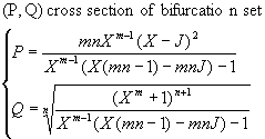
Here we will discuss only the (P, Q) cross section. In (P, Q) cross section the bifuraction set is given by the following expression:
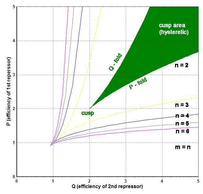
To obtain the bifurcation curve here one should plot the second parameter versus the first, varying X from 0 to P+J. The bifurcation curves for various m and n and no input signal provided are presented in Fig 2.
Figure 2. Bufurcation sets of cross-repressor system for various and equal cooperativity indices. The area of hysteretic behaviour for m=n=2 is filled with green.
The two other cross sections could be viewed by following the links below:
(J, P)-cross section. Behaviour of the system at fixed efficiency Q of the out-of-phase operator.
(J, Q)-cross section. Behaviour of the system at fixed efficiency P of the in-phase operator.
The bifurcation set has a typical cusp geometry. The two lines, leaving the cusp are the two fold catastrophes (they will be real folds if we visualize the response surface). In the region outside the cusp the system is monostable and the response is solely defined by the values of parameters (quasi-stationary). The system (III) has only one positive solution. Inside the cusp the system is bistable. Three roots for system (III) exist, one of them correspond to unstable saddle point – transition state. The dynamic system (II) has to have hysteresis – the responce will depend on the previous history of the process. The amplitude of hysteresis increase rapidly as we get deeper into the cusp region.
The cusp point (the catastrophe itself) deserves some additional words. If we enter the bifurcation set through the cusp point, the number of roots will change from 1 to 3, that is two roots will arise simultaneously (so called pitchfork). With respect to dynamic behaviour, it means that the state of the system will become undetermined. In the cusp point X is the third order root of F. This is the clue point for finding the cusp position. In this point both dP/dX and dQ/dX become zero simultaneously, making d2X/dp1dp2 discontinuous.
In general case, the cusp tip in (P,Q) cross-section of the control space is located at X, given by equation:
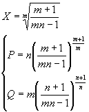
It could not be generally solved. But at J = 0 it could be solved and the cusp position is given by algebraic expression:
There are 3 important findings for J = 0
1. The cusp exists only if m*n>1. At m or n close to 1 the cusp is very narrow, the hysteresis is weak, and could be found only at large P and Q
2. At large m and n the cusp becomes wide and blunt, and asymptotically coincides the quadrant (P>1, Q>1). The latter corresponds to ideal invertors with infinite cooperativities. The hysteresis amplitude is very strong and approaches dynamic range (0, P)
3. The changes of position of the bifurcation set with respect to J become less significant as m*n increase. That is the behavior of the system is most “catastrophic” at intermediate values of m*n (There is a general principle in catastrophe theory stating, that the behavior of the system is more catastrophic when the cusps are sharp).
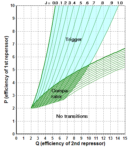
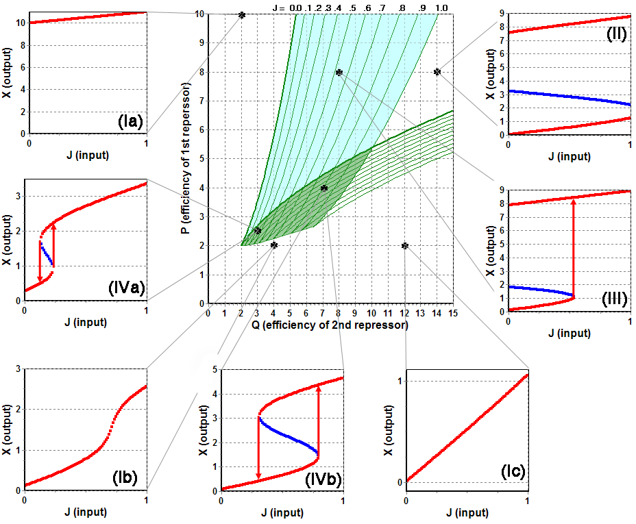
For the selection of P0 and Q0 parameters for the desired device we will consider several cases. (P0 and Q0 are the “efficiencies” of the repressors, that should be used in the device). The positions of the points and typical response curves are shown on figures 3 and 4.
Figure 3. Contour plot of bifurcation set in (P, Q) cross section with J ranging from 0 (thick line) to 1.0 step 0.1 (m=n=2)
I. The (P0, Q0) point is outside the cusp region at all J. This case corresponds to single-value device without hysteresis. If the point is located “below” the cusp catastrophe (Ib) the response may be significantly nonlinear. If it is located “sideways”, the response is monotonous and almost linear. The latter device could hardly have some practical importance.
II. The (P0, Q0) point is inside the cusp region at all available J, so that hysteresis always exist. This device is of no practical importance, as either of its states is maintained infinitely and could not be changed.
III. (Blue area in Figure 3) The (P0, Q0) point is inside the cusp region at J = 0, but exits it at some J1. This case corresponds to full trigger. It will switch to certain state, when J exceeds J1 and will maintain this state at J = 0 and all other positive J. We cannot switch the full trigger back using J input. To do so, we must provide another (reset) input. In our system this could be an addenda to the second equation in (I) similar to J.
IV. (Green area in Figure 3) The (P0, Q0) point is initially outside the cusp region, but it is crossed by both folds of the cusp, while J increases. This case corresponds to a comparator, if the point is located close to the cusp and the hysteresis is narrow (IVa), or Schmitt trigger if the hysteresis is wide (IVb).
Figure 4. Responce curves at selected values of (P0, Q0) for the same case as displayed in Fig. 3. Full trigger, Schmitt trigger as well as linear and nonlinear behaviour could be distinctly seen on the insets. Red points correspond to stable solutions of responce equation (IVb), blue points are unstable solutions, arrows indicate switching transitions
Comment to Figure 4: The responce curves, displayed on fig. 4 could not be obtained by means of pure algebra. To obtain them one should solve Eq. IVb for X using numeric methods. But one could benefit from algebraic analysis, that all roots lie in (0, P+J) interval, and the maximum number of roots is 3, which makes localisation of roots much faster. Stability of the states, corresponding to the roots could be figured out by estimating dX/dJ, which should be positive for stable states.


