ETHZ/Modeling Basics
From 2007.igem.org
| Line 32: | Line 32: | ||
<!--1st drop down menu --> | <!--1st drop down menu --> | ||
<div id="dropmenu_home" class="dropmenudiv_a"> | <div id="dropmenu_home" class="dropmenudiv_a"> | ||
| - | <a href="https://2007.igem.org/wiki/index.php?title=ETHZ#Introduction">Introduction | + | <a href="https://2007.igem.org/wiki/index.php?title=ETHZ#Introduction">Introduction</a> |
| - | <a href="https://2007.igem.org/wiki/index.php?title=ETHZ#Team_Members">Team Members | + | <a href="https://2007.igem.org/wiki/index.php?title=ETHZ#Team_Members">Team Members</a> |
| - | <a href="https://2007.igem.org/wiki/index.php?title=ETHZ#Acknowledgments">Acknowledgments | + | <a href="https://2007.igem.org/wiki/index.php?title=ETHZ#Acknowledgments">Acknowledgments</a> |
| - | <a href="https://2007.igem.org/wiki/index.php?title=ETHZ#Site_Map">Site map | + | <a href="https://2007.igem.org/wiki/index.php?title=ETHZ#Site_Map">Site map</a> |
</div> | </div> | ||
| Line 41: | Line 41: | ||
<!--2nd drop down menu --> | <!--2nd drop down menu --> | ||
<div id="dropmenu_modeling" class="dropmenudiv_a" style="width: 150px;"> | <div id="dropmenu_modeling" class="dropmenudiv_a" style="width: 150px;"> | ||
| - | <a href="https://2007.igem.org/wiki/index.php?title=ETHZ/Model#Introduction">Introduction | + | <a href="https://2007.igem.org/wiki/index.php?title=ETHZ/Model#Introduction">Introduction</a> |
| - | <a href="https://2007.igem.org/wiki/index.php?title=ETHZ/Model#Model_Overview">Model Overview | + | <a href="https://2007.igem.org/wiki/index.php?title=ETHZ/Model#Model_Overview">Model Overview</a> |
| - | <a href="https://2007.igem.org/wiki/index.php?title=ETHZ/Model#Detailed_Model">Detailed Model | + | <a href="https://2007.igem.org/wiki/index.php?title=ETHZ/Model#Detailed_Model">Detailed Model</a> |
| - | <a href="https://2007.igem.org/wiki/index.php?title=ETHZ/Model#Final_Model">Final Model | + | <a href="https://2007.igem.org/wiki/index.php?title=ETHZ/Model#Final_Model">Final Model</a> |
<a href="https://2007.igem.org/wiki/index.php?title=ETHZ/Modeling_Basics">Modeling Basics Page</a> | <a href="https://2007.igem.org/wiki/index.php?title=ETHZ/Modeling_Basics">Modeling Basics Page</a> | ||
| - | <a href="https://2007.igem.org/wiki/index.php?title=ETHZ/Model#Mathematical_Model">Mathematical Model | + | <a href="https://2007.igem.org/wiki/index.php?title=ETHZ/Model#Mathematical_Model">Mathematical Model</a> |
<a href="https://2007.igem.org/wiki/index.php?title=ETHZ/FSM">FSM View Page</a> | <a href="https://2007.igem.org/wiki/index.php?title=ETHZ/FSM">FSM View Page</a> | ||
<a href="https://2007.igem.org/wiki/index.php?title=ETHZ/FlipFlop">Flip-Flop View Page</a> | <a href="https://2007.igem.org/wiki/index.php?title=ETHZ/FlipFlop">Flip-Flop View Page</a> | ||
| Line 54: | Line 54: | ||
<!--3rd drop down menu --> | <!--3rd drop down menu --> | ||
<div id="dropmenu_simulation" class="dropmenudiv_a" style="width: 150px;"> | <div id="dropmenu_simulation" class="dropmenudiv_a" style="width: 150px;"> | ||
| - | <a href="https://2007.igem.org/wiki/index.php?title=ETHZ/Simulation#Introduction">Introduction | + | <a href="https://2007.igem.org/wiki/index.php?title=ETHZ/Simulation#Introduction">Introduction</a> |
| - | <a href="https://2007.igem.org/wiki/index.php?title=ETHZ/Simulation#Simulation_of_Test_Cases">Test Cases | + | <a href="https://2007.igem.org/wiki/index.php?title=ETHZ/Simulation#Simulation_of_Test_Cases">Test Cases</a> |
| - | <a href="https://2007.igem.org/wiki/index.php?title=ETHZ/Simulation#Sensitivity_Analysis">Sensitivity Analysis | + | <a href="https://2007.igem.org/wiki/index.php?title=ETHZ/Simulation#Sensitivity_Analysis">Sensitivity Analysis</a> |
</div> | </div> | ||
<!--4th drop down menu --> | <!--4th drop down menu --> | ||
<div id="dropmenu_biology" class="dropmenudiv_a" style="width: 150px;"> | <div id="dropmenu_biology" class="dropmenudiv_a" style="width: 150px;"> | ||
| - | <a href="https://2007.igem.org/wiki/index.php?title=ETHZ/Biology#Introduction">Introduction | + | <a href="https://2007.igem.org/wiki/index.php?title=ETHZ/Biology#Introduction">Introduction</a> |
| - | <a href="https://2007.igem.org/wiki/index.php?title=ETHZ/Biology#The_Complete_System">The Complete System | + | <a href="https://2007.igem.org/wiki/index.php?title=ETHZ/Biology#The_Complete_System">The Complete System</a> |
| - | <a href="https://2007.igem.org/wiki/index.php?title=ETHZ/Biology#System_Phases">System Phases | + | <a href="https://2007.igem.org/wiki/index.php?title=ETHZ/Biology#System_Phases">System Phases</a> |
<a href="https://2007.igem.org/wiki/index.php?title=ETHZ/Biology/parts">System Parts Page</a> | <a href="https://2007.igem.org/wiki/index.php?title=ETHZ/Biology/parts">System Parts Page</a> | ||
<a href="https://2007.igem.org/wiki/index.php?title=ETHZ/Biology/Lab">Lab Notes Page</a> | <a href="https://2007.igem.org/wiki/index.php?title=ETHZ/Biology/Lab">Lab Notes Page</a> | ||
Revision as of 13:30, 26 October 2007
Modeling Basics
The functioning of our model depends mostly on protein concentrations. These proteins are produced within the E.coli cells, based on genes that we introduced. To understand the system, it is crucial to model the gene expression, gene regulation, and the resulting gene product concentrations accurately.
This Wiki page is intended to present the basic mechanisms and assumptions that went into the mathematical description of our iGEM model.
Constitutive Protein Production
The most simple case, proteins are produced through continuous transcription of genes. At the same time, proteins have a certain half-life time, which means that they are degraded. This leads to the following simple model of protein production/degradation shown in Fig. 1.
To find the concentration of protein P (as a function of time), the system of Fig. 1 can be written as [http://en.wikipedia.org/wiki/Ordinary_differential_equation ordinary differential equation] (ODE):
This equation states that the change of protein concentration is a function of protein production (cmax) and protein degradation (dP[P]).
It is worth looking at the protein production a bit closer: The production of protein P depends on the expression of a gene that codes for this protein. In the case of constant protein production, the gene can be modeled by a constitutive promoter and a coding region for the protein (Fig. 2).
Regulated Protein Production
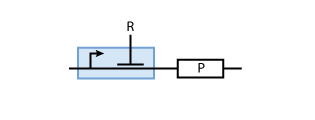
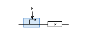
Often, genes are not constitutively expressed but their expression depends on the presence of other proteins R (i.e., transcription factors). These transcription factors can activate or inhibit the promoter of the gene in question. To model such a system, the promoter of the constitutive production system in Fig. 2 must be extended to take into account the presence of the regulatory protein R. Example systems for inhibition and activation of a promoter by R are given in Fig. 3 and Fig.4, respectively.
Inhibition
To derive the equations describing the regulated transcription, we first need a model how the transcription factor interacts with DNA. The most simple model assumes that the protein binds reversibly to the DNA:
Note that the equation above involves n transcription factors. For certain transcription factors the number of proteins involved is indeed greater than 1. These are interesting cases that enable applications such as toggle switches.
When the transcription factor binds to DNA, it blocks the enzymes transcribing the gene. Thus, the higher the concentration of R, the smaller the transcription of the gene. By controlling the concentration of the regulatory protein R, the expression of protein P can effectively be regulated.
To understand this process in more detail, we make the simplification that the binding of R to DNA is in equilibrium. That is, forward and backward reaction rates are identical, so we can write
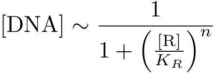
In case of inhibition, the expression of the gene is proportional to the probability that the DNA is 'free' (i.e., there is no transcription factor bound to it). After some algebraic manipulation of the above equation an expression for the 'free DNA' as a function of transcription factor concentration can be derived:
Now, all elements are in place to write down an ODE for the concentration of protein P whose expression is regulated by the regulatory protein R:
The transcription does not always take place at the maximum rate cmax as was the case for the constitutively produced proteins, but is modulated by the concentration of protein R.
Activation
To understand activation, we start with the same assumption: a transcription factor reversibly binding to DNA.
Here, we are interested in the DNA - transcription factor complex because the transcription rate is proportional to the probability that a protein is bound to DNA.
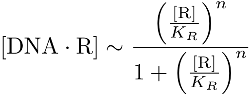
Again assuming equilibrium conditions, we can derive an expression for the DNA-protein complex concentration as a function of protein concentration:
Analogously, we can now write the whole differential equation for protein concentration if transcription is activated by protein R
Basic Production
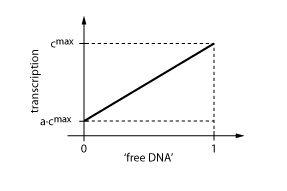
The equations so far assume perfect inhibition/activation. This means, in case of inhibition, that if the inhibitor concentration is high enough, the transcription of protein P is practically zero. Or, in the case of activation, that in the absence of activator protein there is no transcription. In reality, one observes some basic production, despite high inhibitor concentrations or absence of activator protein. The basic transcription is usually around 10-20% of the maximum transcription rate. The case of inhibition is illustrated in Fig. 5.Thus we have to introduce some 'basic transcription' that always takes place. For inhibition we have
and for activation
Note that the basic transcription rate is introduced as a leakiness factor a which is a percentage of the maximum transcription rate cmax. Regulation of transcription by protein R now is only effective in the range between a·cmax and cmax.
Inducer Molecules
A problem in biology is that regulatory proteins (such as protein R in the previous sections) cannot be used as system inputs directly. It is not possible to add such proteins to an assay to steer the behavior of a biological system because these proteins are big and do not diffuse through cell walls. Therefore, they cannot enter the cells.
To circumvent this limitation, one has to produce these proteins directly in the cell. But then, one needs a possibility to switch the functionality of these proteins on and off. This is where inducer molecules become useful. Inducer molecules are small molecules that can diffuse through cell walls freely. Furthermore, they are able to bind to the regulatory proteins and switch the functionality on or off.
Thus, we need a model to describe the binding of the inducer to the protein. We again assume that the inducer I binds reversibly to the protein R
Further on, again we assume that the reaction is in equilibrium. We thus have
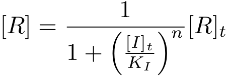
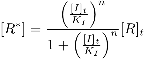
Depending on the species at hand we are either interested in the protein-inducer complex concentration or in the concentration of 'free protein'. For some species (e.g., LuxR), the complex acts as an activator. For others, complex formation relieves repression (e.g., TetR).
It is again possible to derive a formula for both, the concentration of free protein R and the complex concentration R-nI as a function of total inducer concentration (for notational convenience, we write R* for the complex R-nI in the following equations).
Caveats
With this approach to modeling, the equations turn out to be both, easy to understand and to simulate. But to arrive at this point, a certain number of assumptions must be made. This section points out possible problems with these assumptions and ideas to further improve the modeling.
- Equilibrium: This is a very basic assumption that was the basis of all results in the above discussion. At the same time, it is also the least problematic assumption. This can be seen by remembering the massive machinery involved in transcription and translation of DNA/RNA compared to simple reversible binding of molecules. It is plausible to assume that the latter indeed happens on a much shorter time scale than the first.
- Excess of substrate: This assumption was implicitly made when we wrote down the equations of regulation and inducer binding. The basic idea is that the total inducer concentration is very close to the concentration of unbound inducer. Mathematically more precise, this condition is met when KI >> [R]t. As the uncertainty in the values of dissociation constants and steady state concentrations is sometimes very large, it is difficult to say whether this assumption is justified.
- Mechanism dependence: If the [http://en.wikipedia.org/wiki/Hill_coefficient Hill cooperativity coefficient ]n is greater than one, the above formulas become in fact dependent on the mechanism of the binding process. In these cases, the formulas can be off up to a factor n. As the true mechanism of binding is often unknown, it is practically impossible to take this fact into account.
- Low protein concentration. Whenever the concentration is very low (say, below 100 nM in the case of E.coli), the number of molecules per cell becomes small. In this situation, the assumptions behind the ODE modeling approach (e.g., well mixed compartment where each molecule can freely interact with other molecules) are not met any more and simulation results become inaccurate. Then, one would have to resort to stochastic simulations.


