Tokyo/Works/Simulation
From 2007.igem.org
| (One intermediate revision not shown) | |||
| Line 41: | Line 41: | ||
==<!--共存安定になるようなパラメータ範囲の提示-->Determining the range of parameter which satisfy balanced differentiation == | ==<!--共存安定になるようなパラメータ範囲の提示-->Determining the range of parameter which satisfy balanced differentiation == | ||
<!--===The example of coexistent stable state共存安定状態の例=== --> | <!--===The example of coexistent stable state共存安定状態の例=== --> | ||
| - | Depending on the value of parameter | + | Depending on the value of parameter lambda, three different patterns were observed: the pattern with coexistence state of A and B states, the pattern with only A state, and the pattern with only B. The simulation results for their patterns are shown in Fig.1 to 3. |
| - | <!-- | + | <!--パラメータlambdaの値によって,AとBが共存して安定する場合と,Aのみ,Bのみになってしまう3つのパターンが生じる. |
それぞれのパターンについてシミュレーション結果を示すとFig.1-3のようになる.--> | それぞれのパターンについてシミュレーション結果を示すとFig.1-3のようになる.--> | ||
[[Image:3D_start.JPG|200px|left|thumb|Fig.1.A t=0.0(min)]] | [[Image:3D_start.JPG|200px|left|thumb|Fig.1.A t=0.0(min)]] | ||
| Line 51: | Line 51: | ||
[[Image:3D_t30_a.JPG|200px|none|thumb|Fig.1.C t=30(min) only A]] | [[Image:3D_t30_a.JPG|200px|none|thumb|Fig.1.C t=30(min) only A]] | ||
| - | ===[[Tokyo/Works/Simulation/A movie| | + | ===[[Tokyo/Works/Simulation/A movie| ==> movie here!!]]=== |
| Line 60: | Line 60: | ||
[[Image:3D_t30_ab.JPG|200px|none|thumb|Fig.2.C t=30(min) '''A-B balanced differentiation !!''' ]] | [[Image:3D_t30_ab.JPG|200px|none|thumb|Fig.2.C t=30(min) '''A-B balanced differentiation !!''' ]] | ||
| - | ===[[Tokyo/Works/Simulation/AB movie| | + | ===[[Tokyo/Works/Simulation/AB movie| ==> movie here!!]]=== |
[[Image:3D_start.JPG|200px|left|thumb|Fig.3.A t=0.0(min)]] | [[Image:3D_start.JPG|200px|left|thumb|Fig.3.A t=0.0(min)]] | ||
| Line 67: | Line 67: | ||
[[Image:arrow2.JPG|50px|left|thumb]] | [[Image:arrow2.JPG|50px|left|thumb]] | ||
[[Image:3D_t30_b.JPG|200px|none|thumb|Fig.3.C t=30(min) only B]] | [[Image:3D_t30_b.JPG|200px|none|thumb|Fig.3.C t=30(min) only B]] | ||
| - | ===[[Tokyo/Works/Simulation/B movie| | + | ===[[Tokyo/Works/Simulation/B movie| ==> movie here!!]]=== |
<br> | <br> | ||
<!--3パターンについて,nullclinesの交点が2つになる瞬間の相平面はFig.4.A-Cのようになる.--> | <!--3パターンについて,nullclinesの交点が2つになる瞬間の相平面はFig.4.A-Cのようになる.--> | ||
| Line 77: | Line 77: | ||
[[Image:2Dpp-b-tt.JPG|260px|none|thumb|Fig.4.C]] | [[Image:2Dpp-b-tt.JPG|260px|none|thumb|Fig.4.C]] | ||
<br> | <br> | ||
| - | ===[[Tokyo/Works/Simulation/A phase plane movie| | + | ===[[Tokyo/Works/Simulation/A phase plane movie| ==> movie about Fig.4.A here!!]]=== |
| - | ===[[Tokyo/Works/Simulation/A and B phase plane movie| | + | ===[[Tokyo/Works/Simulation/A and B phase plane movie| ==> movie about Fig.4.B here!!]]=== |
| - | ===[[Tokyo/Works/Simulation/B phase plane movie| | + | ===[[Tokyo/Works/Simulation/B phase plane movie| ==> movie about Fig.4.C here!!]]=== |
<br><!--In the case of Fig. 4B, the cell population distributed around the unstable equilibrium point. Right after the moment shown in the Fig. 4B, some cells moved to the A state and the other go in the direction of the B state. The division of the direction may have occurred due to the distribution of the population over the both sides of a “watershed” which is a division line lying over the unstable equilibrium point. In another possibility, fluctuation of the cell state might allow coming or going over the division line.--> | <br><!--In the case of Fig. 4B, the cell population distributed around the unstable equilibrium point. Right after the moment shown in the Fig. 4B, some cells moved to the A state and the other go in the direction of the B state. The division of the direction may have occurred due to the distribution of the population over the both sides of a “watershed” which is a division line lying over the unstable equilibrium point. In another possibility, fluctuation of the cell state might allow coming or going over the division line.--> | ||
| Line 92: | Line 92: | ||
In the case of Fig. 4C, all the cells existed on the B-side across the dividing line from the B-side. Therefore, all the cells were not able to cross over the dividing line and moved to the B state. When all the cells existed on the A-side not the B-side ( Fig 4.A), all the cells moved to the A state, similarly. | In the case of Fig. 4C, all the cells existed on the B-side across the dividing line from the B-side. Therefore, all the cells were not able to cross over the dividing line and moved to the B state. When all the cells existed on the A-side not the B-side ( Fig 4.A), all the cells moved to the A state, similarly. | ||
| - | ===The range of parameter | + | ===The range of parameter lambda <!--範囲の提示-->=== |
| - | <!-- | + | <!--共存安定になるパラメータlambdaの範囲を調べるため,lambdaを変化させてシミュレーションをした.その結果,lambdaの値とAとBが共存安定する確率の関係はFig.5のようになった.--> |
| - | To determine the range of the value of parameter | + | To determine the range of the value of parameter lambda for balanced differentiation, further simulations were carried out by changing the value of lambda. As a result, the relationship between the value of lambda and the probability of balanced differentiation was determined as shown in Fig.5. |
[[Image:range_of_lambda.JPG|400px|thumb|none|Fig.5]] | [[Image:range_of_lambda.JPG|400px|thumb|none|Fig.5]] | ||
| - | <!-- | + | <!--よって,パラメータlambdaをこの範囲の中に入るように調節すれば,我々が目的としているモデルを作り出すことができる!--> |
| - | '''By using parameter | + | '''By using parameter lambda in this range, we can construct the artificial genetic circuit for balanced differentiation!''' It would not be difficult to adjust AHL production efficiency within this range by adjustment of promoter and RBS sequences. |
<br> | <br> | ||
Latest revision as of 05:35, 27 October 2007
Works top 0.Hybrid promoter 1.Formulation 2.Assay1 3.Simulation 4.Assay2 5.Future works
Numerical analysis and kinetic simulations for cell population
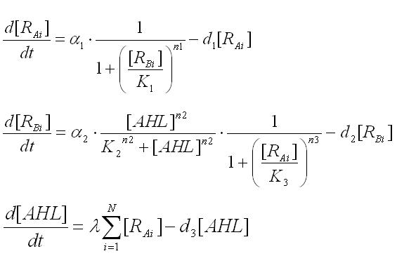
Multi-cell simulations with Hill coefficients of the promoters were carried out to find ranges of other parameters that lead the system to balanced differentiation. The differential equations for N cells were constructed to describe the cell population interacting with each other(Ex3.1).
Here the concentrations of AHL inside and outside of the cell are assumed to be the same since AHL is freely permeable though cell membranes.
First, the phase plane analysis focused on individual cells.
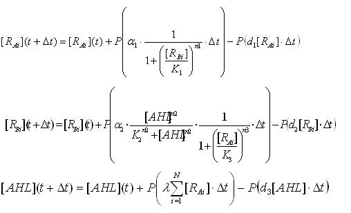
To analyze the behavior of the cell population, the above differential equations for N cells were extended to the stochastic differential equations(Ex3.2). (see detailed derivation ) In order to carry out the simulations with the stochastic model, Poisson random variables were introduced into the differential equations. As a result of the stochastic simulation, the different behaviors of individual cells were observed.
In the simulations, Hill coefficients, coefficients of repression and activation of AHL and LacI(n2,n3,k2,k3) determined by the wet experiments were used. The values of other parameters were determined by reference to some journals. (Kobayashi et al, 2004;Tian T et al, 2006;Garcia-Ojalvo J et al, 2004; Tomioka R et al, 2004)
| n2 | 2.08 (-) |
| K2 | 4.05 (uM) |
| n3 | 2.47 (-) |
| K3 | 0.295 (uM) |
Determining the range of parameter which satisfy balanced differentiation
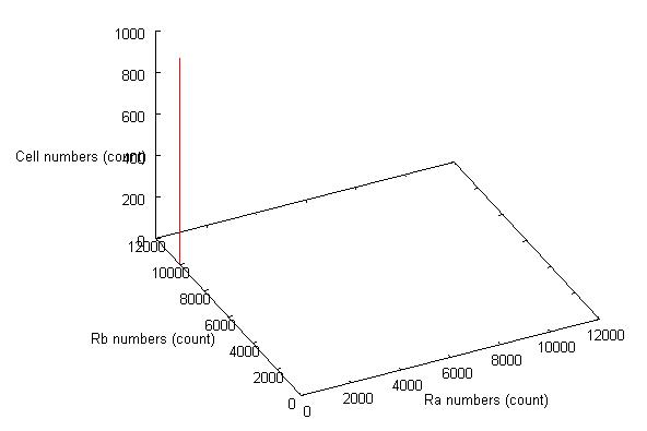
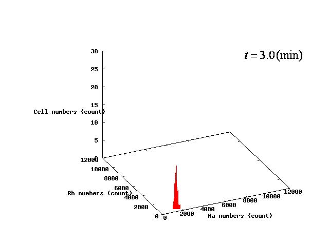
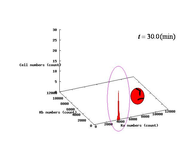
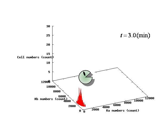
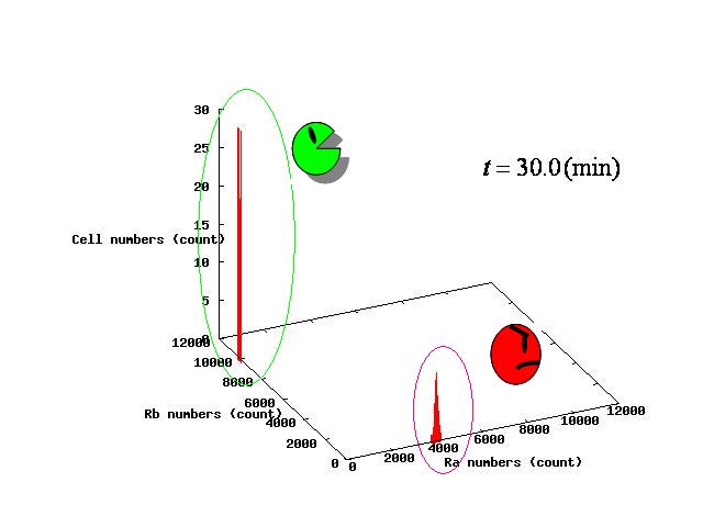
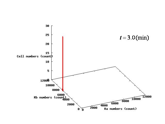
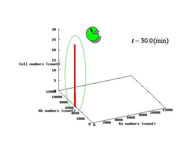
Depending on the value of parameter lambda, three different patterns were observed: the pattern with coexistence state of A and B states, the pattern with only A state, and the pattern with only B. The simulation results for their patterns are shown in Fig.1 to 3.
==> movie here!!
==> movie here!!
==> movie here!!
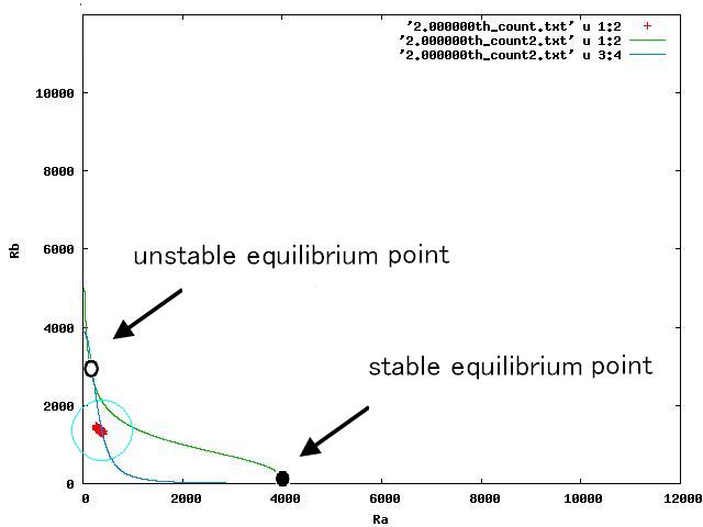
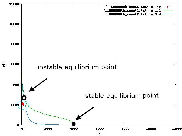
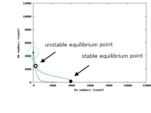
The nullclines changed dependent on the state of the cell population. When there are only B cells, the nullclines had one intersection in the phase plane. As change of the state of the cell population, the number of the intersections of nullclines turned into two. Fig.4.A-C shows the appearance of an additional intersection, indicating an unstable equilibrium point, for the three patterns, respectively.
==> movie about Fig.4.A here!!
==> movie about Fig.4.B here!!
==> movie about Fig.4.C here!!
In Fig. 4B, the cell population was distributed around the unstable equilibrium point. Right after the moment shown in the Fig. 4B, some cells moved to the A state while the others go toward the B state. The division of the direction may have occurred due to the distribution of the population over the both sides of a “watershed,” a division line lying over the unstable equilibrium point. In another possibility, fluctuation of the cell state might allow going across the division line.
In the case of Fig. 4C, all the cells existed on the B-side across the dividing line from the B-side. Therefore, all the cells were not able to cross over the dividing line and moved to the B state. When all the cells existed on the A-side not the B-side ( Fig 4.A), all the cells moved to the A state, similarly.
The range of parameter lambda
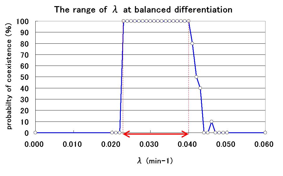
To determine the range of the value of parameter lambda for balanced differentiation, further simulations were carried out by changing the value of lambda. As a result, the relationship between the value of lambda and the probability of balanced differentiation was determined as shown in Fig.5.
By using parameter lambda in this range, we can construct the artificial genetic circuit for balanced differentiation! It would not be difficult to adjust AHL production efficiency within this range by adjustment of promoter and RBS sequences.
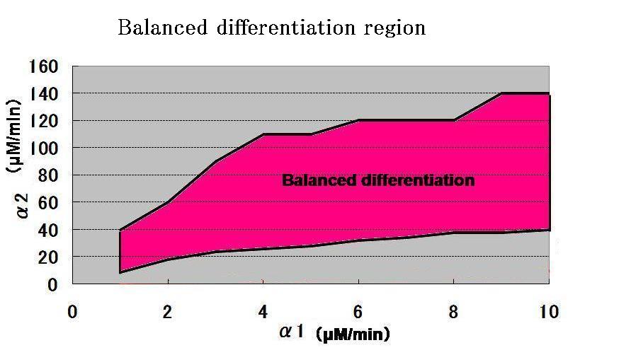
In addition, from the result of simulation, it was found that when the value of parameter lambda was fixed, the value of parameter ALPHA2 is needed to be greater than that of ALPHA1, for the balanced differentiation of the system.(ALPHA1,ALPHA2 represent the expression rate of Ra and Rb respectively)
supplementary data Click here!!
