From 2007.igem.org

Revision as of 19:29, 22 October 2007

Introduction

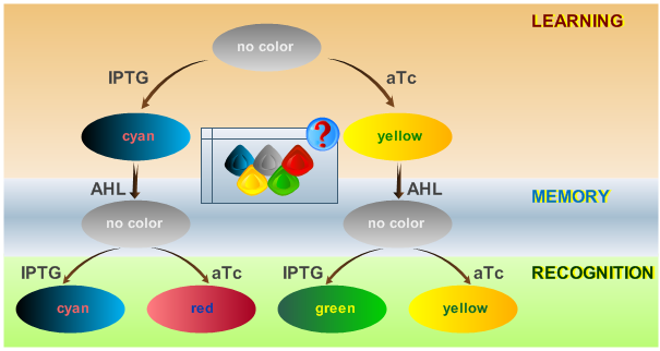
As has been presented in the Modeling page, we have created a model of our system that can be described as a finite state machine. In order to examine the behavior of our system thoroughly, we have to simulate it through all the difference phases that can be reached. We carry out our simulations based on the protocol presented in Fig. 1.

Fig. 1: Flow diagram. This figure shows the protocol with which the final system should be tested, as well as the test results in the form of the reported colors. There are three phases the system has to go through: (1) a training or learning phase in which the system learns an input and stores it in its memory, (2) a memory phase in which the system has to keep the content of its memory and, (3) a recognition phase where the output of the system depends on the content of its memory as well as on the current input.

Simulation of Test Cases

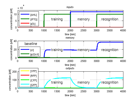
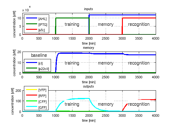
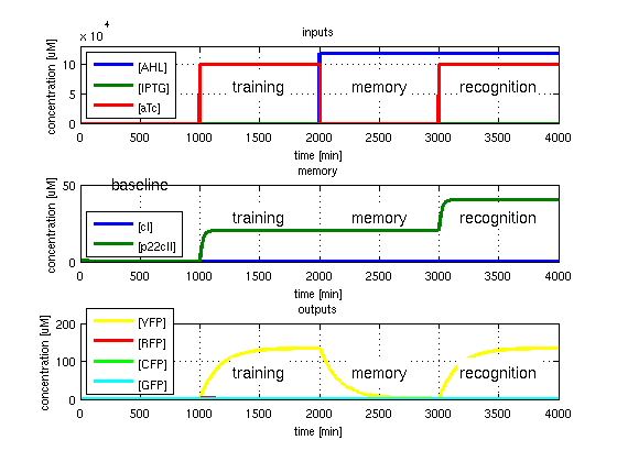
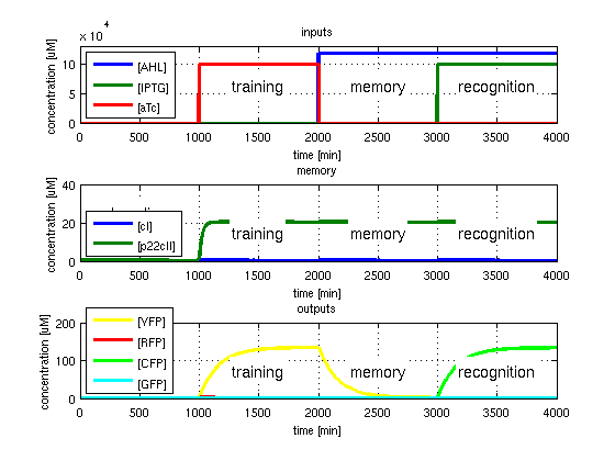
To test all the possible conditions and transitions in our system, we run timing simulations for all 4 different branches in the flow diagram of our protocol, and we plot the concentrations of the inducers, memory proteins and reporter proteins. During each learning, memorizing and recognizing phase, we wait for the steady state of the system to be reached. The three phases of the system are thus separated sufficiently in time. In all the cases, we follow the following procedure:

• During the first 1000 minutes of the simulation, we do not add any inducers to the system, and as a result, we check for the baseline production of proteins.
• Between 1000 and 2000 minutes, we add the inducer that should be learned, and we let the system reach steady state.
• After 2000 minutes, we add the inducer AHL for memory formation, and run the simulation for an additional 1000 minutes, to reach again steady state.
• Between 3000 and 4000 minutes, we test the final behavior of the system, and check if it reacts in the desired way, by showing the appropriate color.

The parameters of the system are crucial if one wants to have accurate and realistic simulations. We present the parameters used to simulate our system, in the section Parameters.

Fig. 2: Test case 1 - Learn and recognize IPTG. The simulated behavior of the system, when IPTG is presented both during the learning phase, and the recognition phase. In both the learning and recognition phase, the system reports by producing CFP, which matches the desired behavior.

Fig. 3: Test case 2 - Learn IPTG and get tested for aTc. The simulated behavior of the system, when IPTG is presented during the learning phase, and aTc is presented during the recognition phase. The system reports by producing RFP during the recognition phase, which matches the desired behavior.

Fig. 4: Test case 3 - Learn and recognize aTc. The simulated behavior of the system, when aTc is presented both during the learning phase and the recognition phase. In both the learning and recognition phase the system reports by producing YFP, which matches the desired behavior.

Fig. 5: Test case 4 - Learn aTc and get tested for IPTG. The simulated behavior of the system, when aTc is presented during the learning phase, and IPTG is presented during the recognition phase. The system reports by producing GFP during the recognition phase, which matches the desired behavior.

Sensitivity Analysis

In order for one to ensure a biological system will operate as it was modeled, he/she should understand the sensitivity of the system's behavior to all involved parameters. Due to the uncertainty in parameter retrieval, we would like our system to have reduced sensitivity to the parameters that are affected mostly by noise. That way, we can have a guaranteed stable performance, even under non-simulated conditions.

Fig. 5: Sensitivity analysis

We simulated the behavior of our system throughout all its phases, while sweeping the parameters by 5%, one at a time. More specifically for the case presented in Fig. 1, we carried out the following procedure: For each parameter, we did the timing simulation as shown in Fig. 2. Once we increased the parameter by 5%, and once we decreased the parameter by 5%. Since in test case 1 (Fig. 2) we are interested in having a high concentration of CFP during the recognition phase with respect to the base line, we divide the steady state CFP concentration at 4000 minutes by the baseline concentration at 1000 minutes. Finally, as shown in the following equation, we define the sensitivity by subtracting the resulting factor that we get with an increased parameter, from the resulting factor that we get by a decreased parameter.

We can summarize that, if there is no difference in the concentration of the desired output during the recognition phase with respect to baseline when sweeping a parameter by +/-5%, the sensitivity of that parameter is equal to zero. Otherwise the sensitivity gives us a measure of how much the concentration changes.

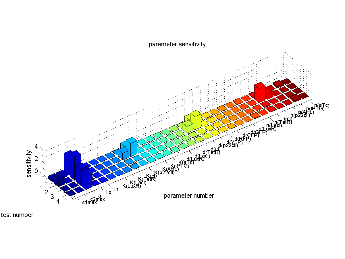
We quantified the sensitivity for all parameters and test cases. The results are plotted in Fig. 5.

The conclusions that can be derived from our sensitivity analysis are the following:

• Our system is most sensitive to the parameter "a", which describes the base production. This is not a surprising result, since we depend on having a good switch, and our signal-to-noise ratio, or output to baseline production level, depends highly on the fact that we can reliably switch off the production of the memory proteins cI and p22cII. For a more detailed analysis of the switching behavior please see our biological implementation page.
• Other sensitive parameters are those that are directly related to the production and decay of the memory proteins cI and p22cII. This can be explained by the fact that our system prefers symmetry between the parameter sets of cI and p22cII, in order to support good switching behavior where the same concentration of p22cII leads to the same repression of cI and vice versa. We can especially see that those parameters seem to be more sensitive for the test cases 1 and 2, where cI has to be stored inside the memory. The reason for this behavior is due to the missing symmetry between the parameters for cI and p22cII, we currently have a bias inside the system towards the production of p22cII.