From 2007.igem.org

Revision as of 22:11, 23 October 2007

Introduction

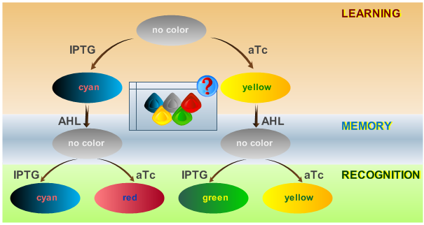
As has been presented in the Modeling page, we have created a model of our system that can be described as a finite state machine. In order to examine the behavior of our system thoroughly, we have to simulate it through all the difference phases that can be reached. We carry out our simulations based on the protocol presented in Fig. 1.

Fig. 1: Flow diagram. This figure shows the protocol with which the final system should be tested, as well as the test results in the form of the reported colors. There are three phases the system has to go through: (1) a training or learning phase in which the system learns an input and stores it in its memory, (2) a memory phase in which the system has to keep the content of its memory and, (3) a recognition phase where the output of the system depends on the content of its memory as well as on the current input.

Simulation of Test Cases

To test all the possible conditions and transitions in our system, we run timing simulations for all 4 different branches in the flow diagram of our protocol, and we plot the concentrations of the inducers, memory proteins and reporter proteins. During each learning, memorizing and recognizing phase, we wait for the steady state of the system to be reached. The three phases of the system are thus separated sufficiently in time. In all the cases, we follow the following procedure:

• During the first 1000 minutes of the simulation, we do not add any inducers to the system, and as a result, we check for the baseline production of proteins.
• Between 1000 and 2000 minutes, we add the inducer that should be learned, and we let the system reach steady state.
• After 2000 minutes, we add the inducer AHL for memory formation, and run the simulation for an additional 1000 minutes, to reach again steady state.
• Between 3000 and 4000 minutes, we test the final behavior of the system, and check if it reacts in the desired way, by showing the appropriate color.

The parameters of the system are crucial if one wants to have accurate and realistic simulations. We present the parameters used to simulate our system, in the section Parameters.

Fig. 2: Test case 1 - Learn and recognize IPTG. The simulated behavior of the system, when IPTG is presented both during the learning phase, and the recognition phase. In both the learning and recognition phase, the system reports by producing CFP, which matches the desired behavior.

Fig. 3: Test case 2 - Learn IPTG and get tested for aTc. The simulated behavior of the system, when IPTG is presented during the learning phase, and aTc is presented during the recognition phase. The system reports by producing RFP during the recognition phase, which matches the desired behavior.

Fig. 4: Test case 3 - Learn aTc and get tested for IPTG. The simulated behavior of the system, when aTc is presented during the learning phase, and IPTG is presented during the recognition phase. The system reports by producing GFP during the recognition phase, which matches the desired behavior.

Fig. 5: Test case 4 - Learn and recognize aTc. The simulated behavior of the system, when aTc is presented both during the learning phase and the recognition phase. In both the learning and recognition phase the system reports by producing YFP, which matches the desired behavior.

Sensitivity Analysis

Before performing simulations we did an intensive literature review to find the parameters of our system. Due to the uncertainty in parameter retrieval, we would like our system to have reduced sensitivity to the parameters. That way, we can have a guaranteed stable performance, even under non-simulated conditions.

Fig. 6: Sensitivity analysis. We plot the sensitivity for each parameter and each test case that corresponds to the different path ways in Fig. 1.

We define sensitivity as the change of the production of the desired florescence protein - which corresponds to the output of our system - depending on the change of the parameters. As shown in Fig. 1 the desired florescence protein output depends on the inducers that we present to our system during learning and recognition phase. Overall we have 4 different combinations leading to the 4 different test cases shown in Fig. 1. E.g. when IPTG is presented to the system both during the learning and recognition phase we expect the production of CFPs. That is why we define the sensitivity for test case 1 as

where

• [CFP_recognition^105%] describes the concentration of CFP during the recognition phase when the parameter that we test for is increased by 5%,
• [CFP_baseline^105%] describes the concentration of CFP without any inducers given to the system when the parameter that we test for is increased by 5%,
• [CFP_recognition^95%] describes the concentration of CFP during the recognition phase when the parameter that we test for is decreased by 5%, and
• [CFP_baseline^95%] describes the concentration of CFP without any inducers given to the system when the parameter that we test for is decreased by 5%.

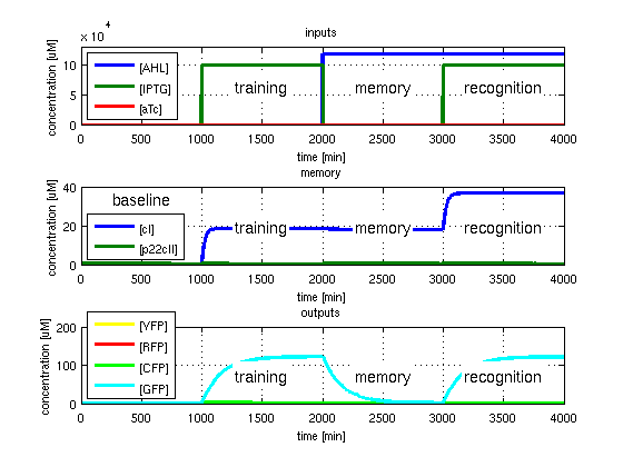
All concentrations are gained from timing simulations as shown in Fig. 2 when the concentrations reached steady state. E.g. [CFP_recognition] corresponds to the value of CFP after 4000 minutes while [CFP_baseline] is equal to the value for CFP after 1000 minutes.

We define sensitivity by using the ratio of [CFP_recognition] and [CFP_baseline] to see by which factor the CFP concentration is increased during the recognition phase. The higher this value is the easier it will be possible to determine the correct readout.

We subtract the two ratios of [CFP_recognition]/[CFP_baseline] for increasing and decreasing the parameter under test by 5% to quantify how much is the influence of the parameter on the output. If the output ratio does not change the parameter has no influence and the sensitivity is equal to zero.

We quantified the sensitivity for all parameters and all 4 test cases. Therefor we look at the concentration of

• CFP in test case 1. A timing simulation for this case is shown in Fig. 2.
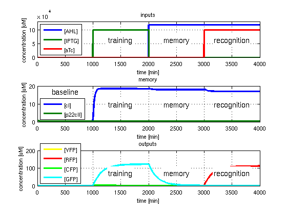
• RFP in test case 2. A timing simulation for this case is shown in Fig. 3.
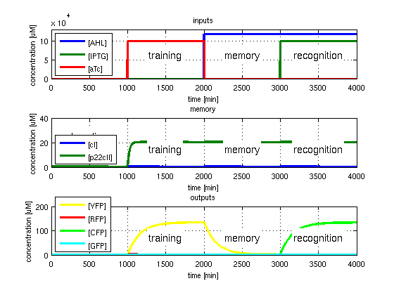
• YFP in test case 3. A timing simulation for this case is shown in Fig. 4.
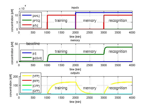
• GFP in test case 4. A timing simulation for this case is shown in Fig. 5.

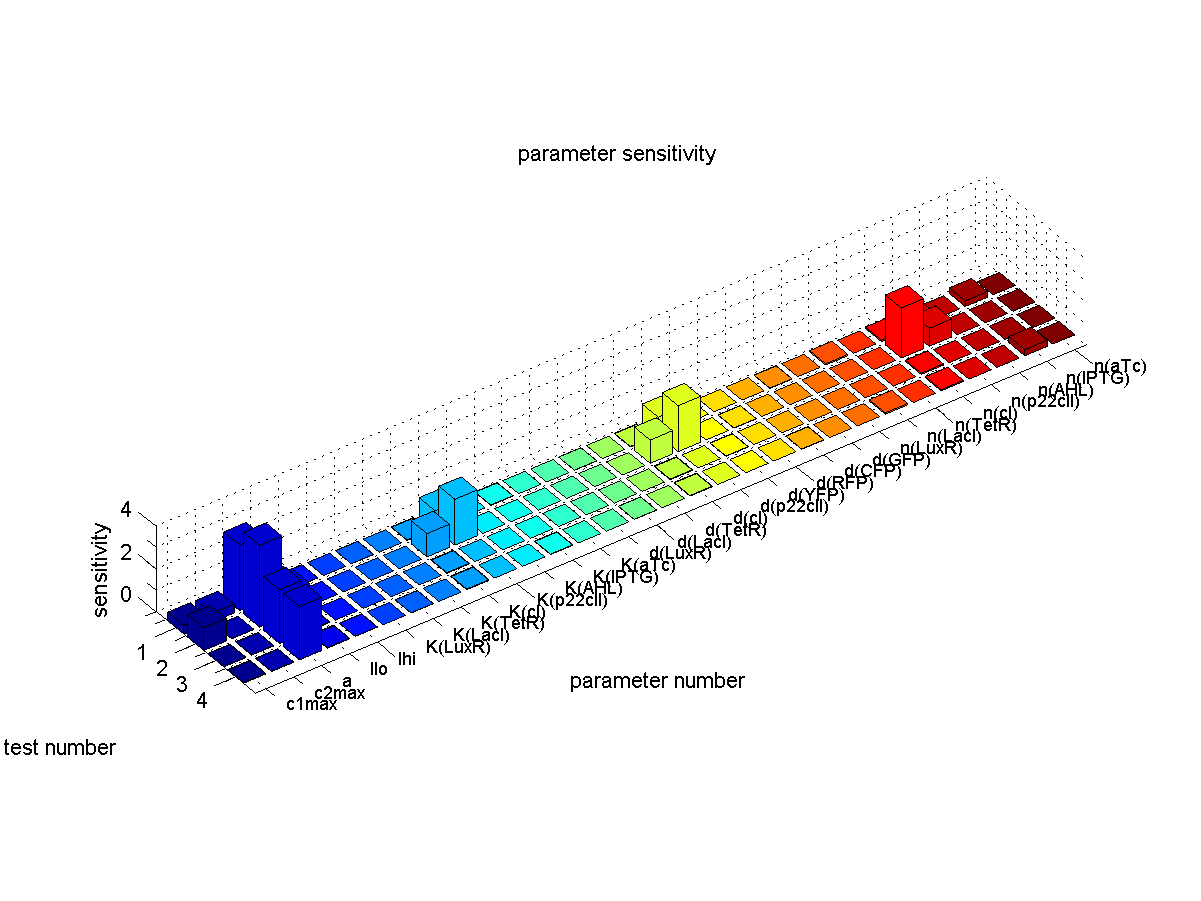
The results are plotted in Fig. 6. Furthermore we make sure that no undesired florescence protein is produced during the recognition phase.

The conclusions that can be derived from our sensitivity analysis are the following:

• Most of the parameters are not sensitive which corresponds to the desired behavior since the system should ideally give a constant output for the same input sequence.
• Our system is most sensitive to the parameter "a", which describes the base production. This is not a surprising result, since we depend on having a good switch. However, we cannot reliably switch off the production of the memory proteins cI and p22cII. This leads to a small signal to noise ration and in the worst case the memory does not work at all. For a more detailed analysis of the switching behavior please see our biological implementation page.
• Other sensitive parameters are those that are directly related to the production and decay of the memory proteins cI and p22cII. This can be explained by the fact that our system prefers symmetry between the parameter sets of cI and p22cII, in order to support good switching behavior where the same concentration of p22cII leads to the same repression of cI and vice versa. We can especially see that those parameters seem to be more sensitive for the test cases 1 and 2, where cI has to be stored inside the memory. The reason for this behavior is due to the missing symmetry between the parameters for cI and p22cII, we currently have a bias inside the system towards the production of p22cII.