Tokyo/Works/Simulation
From 2007.igem.org
(→シミュレーションはpopulationモデルに拡張し,確率微分方程式を用いた) |
|||
| Line 3: | Line 3: | ||
<!--==ここまでわかったこと==--> | <!--==ここまでわかったこと==--> | ||
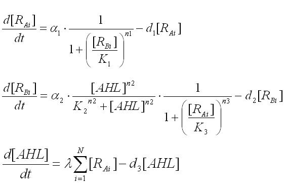
| - | + | Multi-cell simulations with Hill coefficients of the promoters were carried out to find ranges of other parameters that lead the system to balanced differentiation. The differential equations for N cells were constructed to describe the cell population interacting with each other(Ex3.1). | |
| + | '''[[Tokyo/Formulation/4.population model| ⇒ see more]]''' | ||
| - | |||
| - | |||
| - | |||
| - | |||
| - | |||
| - | |||
[[Image:expression4-1.jpg|300px|thumb|none|Ex3.1 the differential equations of population model]] | [[Image:expression4-1.jpg|300px|thumb|none|Ex3.1 the differential equations of population model]] | ||
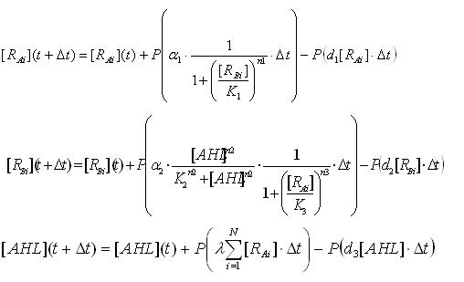
| - | + | To analyze the behavior of the cell population, the above differential equations for N cells were extended to the stochastic differential equations(Ex3.2). In order to carry out the simulations with the stochastic model, Poisson random variables were introduced into the differential equations. As a result of the stochastic simulation, the different behaviors of individual cells were observed. | |
| - | + | ||
| - | + | ||
| - | + | ||
<br>[[Image:expression5-1.jpg|400px|thumb|none|Ex3.2 the stochastic differential equations of the population model]] | <br>[[Image:expression5-1.jpg|400px|thumb|none|Ex3.2 the stochastic differential equations of the population model]] | ||
| - | |||
| - | |||
| - | |||
| - | |||
== What we have found so far == | == What we have found so far == | ||
Revision as of 17:32, 26 October 2007
Works top 0.Hybrid promoter 1.Formulation 2.Assay1 3.Simulation 4.Assay2 5.Future works
Multi-cell simulations with Hill coefficients of the promoters were carried out to find ranges of other parameters that lead the system to balanced differentiation. The differential equations for N cells were constructed to describe the cell population interacting with each other(Ex3.1). ⇒ see more
To analyze the behavior of the cell population, the above differential equations for N cells were extended to the stochastic differential equations(Ex3.2). In order to carry out the simulations with the stochastic model, Poisson random variables were introduced into the differential equations. As a result of the stochastic simulation, the different behaviors of individual cells were observed.
What we have found so far
Wet experiments have determined Hill coefficients, coefficients of repression and activation of AHL and LacI(n2,n3,k2,k3) as follows.
n2 = 2.08 (-)
K2 = 4.05 (μM)
n3 = 2.47 (-)
K3 = 0.295 (μM)
Determining the range of parameter which satisfy coexistent stability
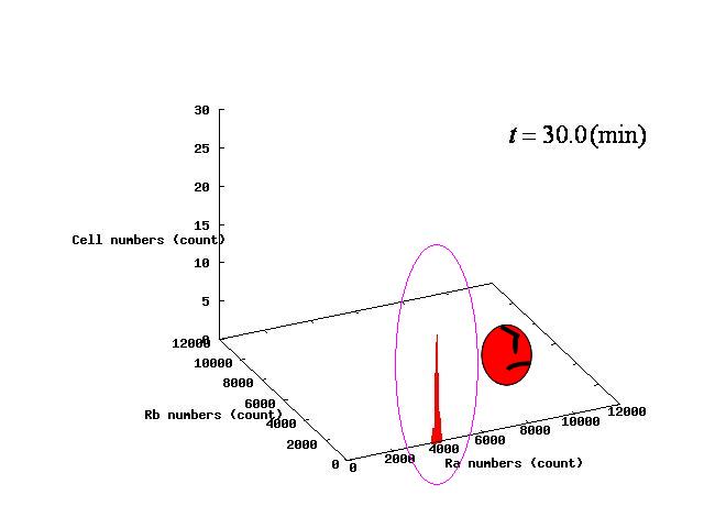
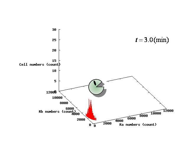
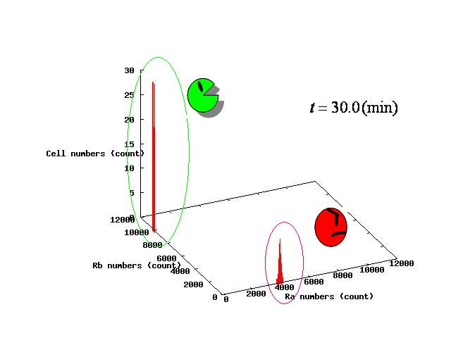
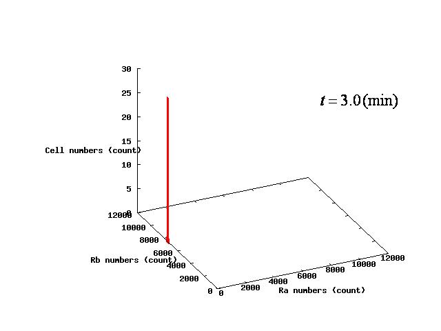
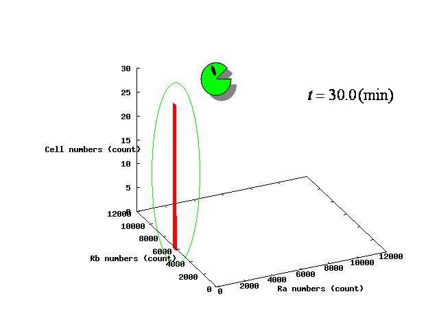
The example of coexistent stable state
⇒ movie here!!
⇒ movie here!!
⇒ movie here!!
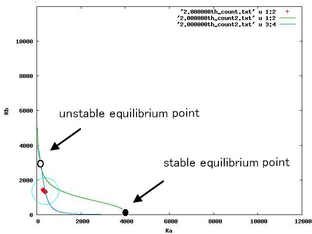
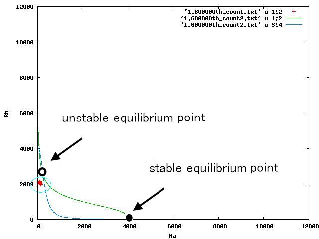
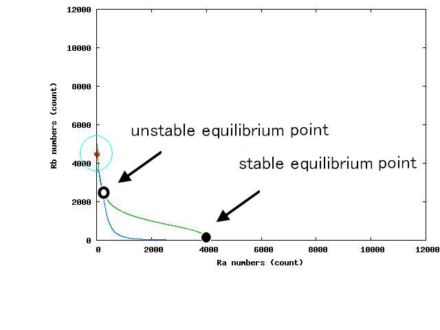
For the three patterns, the phase portraits at the moment when the number of the intersection of nullclines become two are shown in Fig.4.A-C respectively.
Fig.4.A shows that when the two equilibrium points appeared, cells were existing closer to A-side than the unstable equilibrium point. Oppositely,in Fig.4.C,when the two equilibrium points appeared, cells were existing closer to A-side than the unstable equiliblium point. Since when the number of the intersection of nullclines becomes two, stable point appears on B-side, at the moment of Fig.4, cells on the A-side cannot transit to B-side across unstble equilibrium point. As a result, all cells transit to A-side.
⇒ movie about Fig.4.A here!!
⇒ movie about Fig.4.B here!!
⇒ movie about Fig.4.C here!!
The range of parameter λ
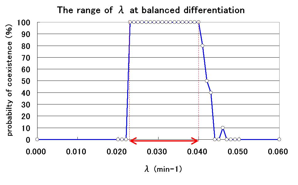
To determine the range of parameter λ, several simulations were conducted with different values of λ. As a result, the relationship between λ value and the probability of coexistence is determined as shown in Fig.5.
By using parameter λ in this range, we can construct our model.
