Tokyo/Formulation/1.toggle model
From 2007.igem.org
| (36 intermediate revisions not shown) | |||
| Line 1: | Line 1: | ||
| - | + | __NOTOC__ | |
| - | + | <br>[[Tokyo/Works|Works top]] 0.[[Tokyo/Works/Hybrid promoter|Hybrid promoter]] '''1.[[Tokyo/Works/Formulation |Formulation]]''' 2.[[Tokyo/Works/Assay |Assay1]] 3.[[Tokyo/Works/Simulation |Simulation]] 4.[[Tokyo/Works/Assay2 |Assay2]] 5.[[Tokyo/Works/Future works |Future works]] | |
| - | + | <br><br>[[Tokyo/Formulation/1.toggle model |Step1]] [[Tokyo/Formulation/2.toggle model with hybrid promoter |Step2]] [[Tokyo/Formulation/3.AHL-experssing model|Step3]] | |
| - | + | <br> | |
| - | + | == 1.Single cell model:mutual inhibition == | |
| - | + | First, the ordinary differential equations (ODEs) of the toggle switch were derived as | |
| + | <br>[[Image:expression1-1.jpg|200px|left|thumb|Ex1-1 ]] [[Image:parameter1-1.jpg|200px|]] | ||
| - | <br> | + | <br>These equations were normalized as follows: |
| - | <br> | + | <br>[[Image:expression1-2.jpg|200px|none|thumb|Ex1-2 ]] |
| - | <br> | + | <br>In the steady state, time derivatives are zero: |
| - | <br> | + | <br>[[Image:expression1-3.jpg|80px|none|thumb|Ex1-3]] |
| - | + | ||
| - | <br> | + | <br>As a result, the nullclines of this system were derived as |
| - | <br> | + | <br>[[Image:Siki2.jpg|200px|none|thumb|Ex1-4]] |
| - | + | ||
| - | + | ||
| - | <br> | + | <br>which indicate the nullclines of the system shown in Fig 1.1.A-C. Where about parameters, we use three sets of parameters. |
| - | <br> | + | <br> A)the maximum expression rate of repressor A and repressor B is balanced,and hill coefficient of both A and B is three. |
| - | + | <br>[[Image:parameter1-2.jpg|150px|center|thumb|Table1.A]] | |
| + | <br> B)the maximum expression rate of repressor A and repressor B is equal,and hill coefficient of A is one. | ||
| + | <br>[[Image:parameter1-3.JPG|150px|center|thumb|Table1.B]] | ||
| + | <br> C)the maximum expression rate of repressor A and repressor B is not balanced,and hill coefficient of both A and B is three. | ||
| + | <br>[[Image:parameter1-4.JPG|150px|center|thumb|Table1.C]] | ||
| - | <br> | + | [[Image:toggle1.jpg|260px|left|thumb|Figure 1.1.A]] |
| + | [[Image:toggle2.jpg|270px|left|thumb|Figure 1.1.B]] | ||
| + | [[Image:Toggle1-4.jpg|270px|none|thumb|Figure 1.1.C]] | ||
| + | <br>First,we carried out kinetic simulations in the condition of Fig 1.1.A. The results are shown in Fig 1.2.A-C. | ||
| + | |||
| + | [[Image:toggle3.jpg|200px|left|thumb|Figure 1.2.A (Ra(0),Rb(0))=(0.0,2.5)]] [[Image:toggle4.JPG|200px|left|thumb|Figure 1.2.B (Ra(0),Rb(0))=(2.5,0.0)]] | ||
| + | [[Image:toggle5.JPG|200px|left|thumb|Figure 1.2.C (Ra(0),Rb(0))=(1.5,1.3)]] | ||
| + | [[Image:toggle1-1.jpg|200px|none|thumb|Figure 3 bistable]] | ||
| + | |||
| + | |||
| + | <br>Fig 1.2.A-C indicate that when the initial condition is (Ra,Rb)=(0.0,2.5), which is near the stable equilibrium point B, the values of Ra and Rb go to stable equilibrium point B, and when the initial condition is (Ra,Rb)=(2.5,0.0), which is near the stable equilibrium point A, the values of Ra and Rb go to the stable equilibrium point B. | ||
| + | |||
| + | <br>Next, when the number of stable equilibrium point is one(Fig 1.1.B), the result of simulation are shown in Fig 1.4.A-C. | ||
| + | |||
| + | [[Image:toggle6.JPG|200px|left|thumb|Figure 1.4.A (Ra(0),Rb(0))=(0.0,2.5)]] [[Image:toggle7.JPG|200px|left|thumb|Figure 1.4.B (Ra(0),Rb(0))=(2.5,0.0)]] | ||
| + | [[Image:toggle8.JPG|200px|left|thumb|Figure 1.4.C (Ra(0),Rb(0))=(1.5,1.3)]] | ||
| + | [[Image:toggle1-2.jpg|220px|none|thumb|Figure 1.5 monostable]] | ||
| + | |||
| + | <br><br> | ||
| + | <br> | ||
| + | <br>Fig 4.A-C indicate that the value of Ra and Rb go to the stable equilibrium point A regardless of an initial value in case of monostable state. | ||
| + | |||
| + | <br>'''As a result, taking two stable states needs the phaseplane of two stable equilibrium points and Hill coefficients was very important.''' | ||
| + | |||
| + | == == | ||
| + | [[Tokyo/Formulation/1.toggle model|Step.1]] >> [[Tokyo/Formulation/2.toggle model with hybrid promoter|Step.2]] | ||
Latest revision as of 02:45, 27 October 2007
Works top 0.Hybrid promoter 1.Formulation 2.Assay1 3.Simulation 4.Assay2 5.Future works
Step1 Step2 Step3
1.Single cell model:mutual inhibition
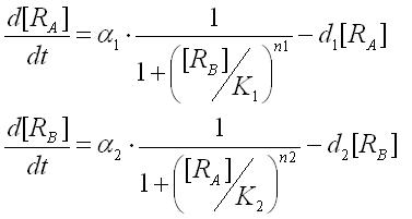
First, the ordinary differential equations (ODEs) of the toggle switch were derived as
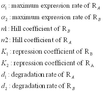
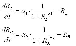
These equations were normalized as follows:
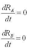
In the steady state, time derivatives are zero:
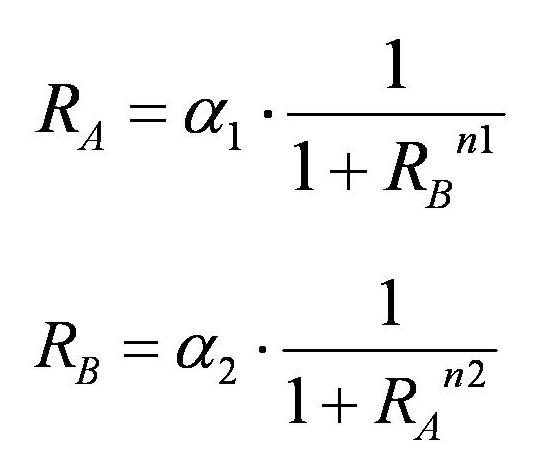
As a result, the nullclines of this system were derived as
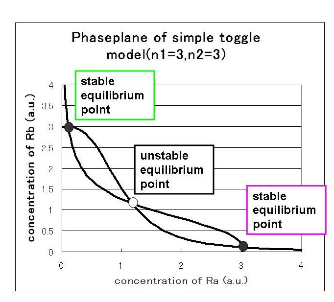
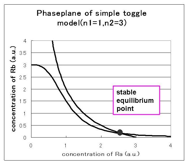
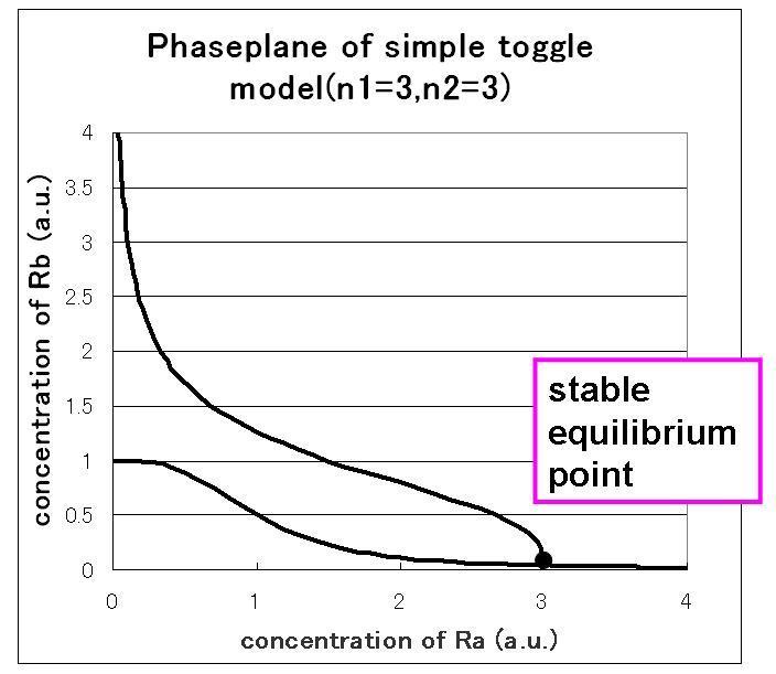
which indicate the nullclines of the system shown in Fig 1.1.A-C. Where about parameters, we use three sets of parameters.
A)the maximum expression rate of repressor A and repressor B is balanced,and hill coefficient of both A and B is three.
B)the maximum expression rate of repressor A and repressor B is equal,and hill coefficient of A is one.
C)the maximum expression rate of repressor A and repressor B is not balanced,and hill coefficient of both A and B is three.
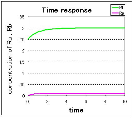
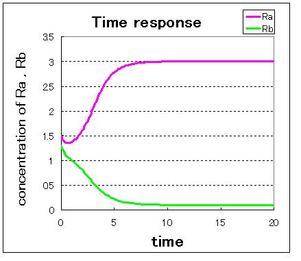
First,we carried out kinetic simulations in the condition of Fig 1.1.A. The results are shown in Fig 1.2.A-C.
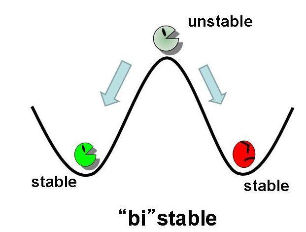
Fig 1.2.A-C indicate that when the initial condition is (Ra,Rb)=(0.0,2.5), which is near the stable equilibrium point B, the values of Ra and Rb go to stable equilibrium point B, and when the initial condition is (Ra,Rb)=(2.5,0.0), which is near the stable equilibrium point A, the values of Ra and Rb go to the stable equilibrium point B.
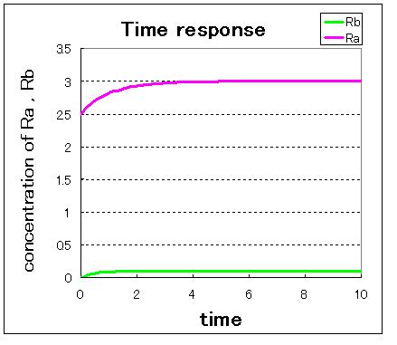
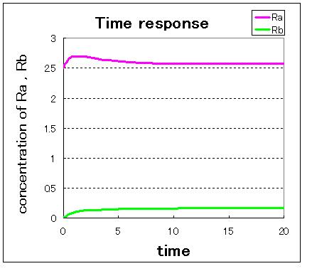
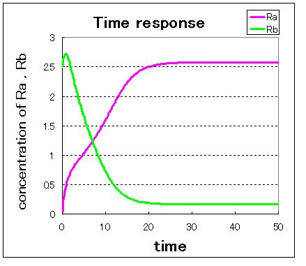
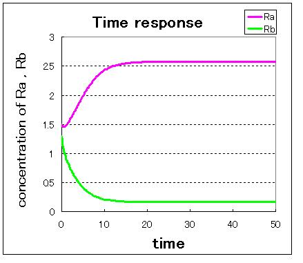
Next, when the number of stable equilibrium point is one(Fig 1.1.B), the result of simulation are shown in Fig 1.4.A-C.
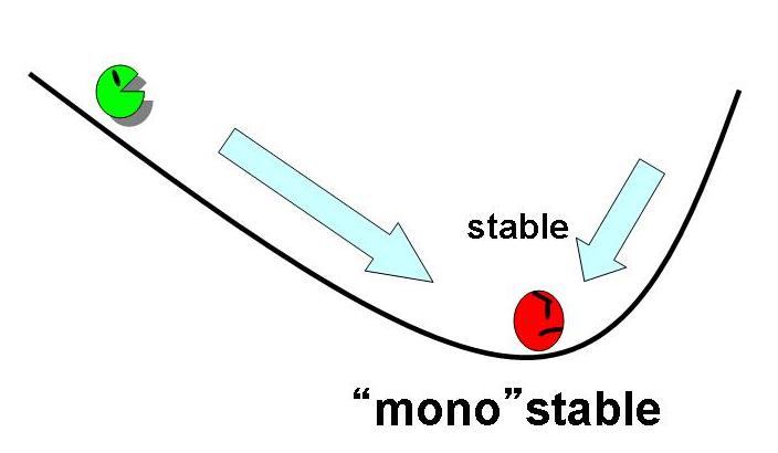
Fig 4.A-C indicate that the value of Ra and Rb go to the stable equilibrium point A regardless of an initial value in case of monostable state.
As a result, taking two stable states needs the phaseplane of two stable equilibrium points and Hill coefficients was very important.
Step.1 >> Step.2
