Imperial/Cell-Free/Characterisation
From 2007.igem.org
m (→Temperature Dependence of the Synthesis Rate) |
|||
| (38 intermediate revisions not shown) | |||
| Line 1: | Line 1: | ||
{{Template:IC07navmenu}} | {{Template:IC07navmenu}} | ||
__NOTOC__ | __NOTOC__ | ||
| + | <html> | ||
| + | <link rel="stylesheet" href="/igem07/index.php?title=User:Dirkvs/Stylesheets/IC07persist.css&action=raw&ctype=text/css" type="text/css" /> | ||
| + | |||
| + | <div id="tabs"> | ||
| + | <ul> | ||
| + | <li><a href="https://2007.igem.org/Imperial/Cell-Free/Whatis" title=""><span>What is Cell-Free?</span></a></li> | ||
| + | <li><a href="https://2007.igem.org/Imperial/Cell-Free/Comparison" title=""><span>Advantages of CFS</span></a></li> | ||
| + | <li><a href="https://2007.igem.org/Imperial/Cell-Free/Contribution" title=""><span>Our Contributions</span></a></li> | ||
| + | <li><a class="current" href="https://2007.igem.org/Imperial/Cell-Free/Characterisation" title=""><span>Characterisation</span></a></li> | ||
| + | <li><a href="https://2007.igem.org/Imperial/Cell-Free/Applications" title=""><span>CFS Applications</span></a></li> | ||
| + | |||
| + | </ul> | ||
| + | </div> | ||
| + | <hr /> | ||
| + | <br clear="all"> | ||
| + | </html> | ||
= Cell-Free: Characterisation = | = Cell-Free: Characterisation = | ||
| + | |||
| + | |||
== Introduction == | == Introduction == | ||
| - | + | ||
| - | In this section we analyse the data we have obtained on the cell-free chassis using GFP as the reporter. We show that the classic model for the synthesis of a protein by a constitutive promoter is not adapted and introduce a new model where synthesis is curbed by the resources left in the system. Finally we estimate the parameters of this new model from our data and show that it yields a much better fit. | + | In this section we analyse the data we have obtained on the cell-free chassis using GFP as the reporter. We show that the classic model for the synthesis of a protein by a constitutive promoter is not adapted and introduce a new model where synthesis is curbed by the resources left in the system. We also introduce an Arrhenius vision of the temperature dependence of sysnthesis rate. Finally we estimate the parameters of this new model from our data and show that it yields a much better fit. |
=== Prior Knowledge === | === Prior Knowledge === | ||
* pTet and pT7 are constitutive promoters that are commonly used ''in vivo'' for ''E. coli'' | * pTet and pT7 are constitutive promoters that are commonly used ''in vivo'' for ''E. coli'' | ||
| - | * [[Imperial/Wet_Lab/ | + | * [[Imperial/Wet_Lab/Results/CBD1.2|Tests]] ''in vitro'' have demonstrated that they also work on the cell-free chassis |
* Manufacturer specifications: the solution has been optimised so the degradation of proteins is minimal. We therefore expect our analysis to find very small degradation terms | * Manufacturer specifications: the solution has been optimised so the degradation of proteins is minimal. We therefore expect our analysis to find very small degradation terms | ||
| Line 16: | Line 34: | ||
For this section we will use | For this section we will use | ||
| - | * the data collected with pTet at 4,15,25 and 37 degrees | + | * the [[Imperial/Wet_Lab/Results/CBD2.2|data]] collected with pTet at 4,15,25 and 37 degrees that exhibit a linear behaviour |
| - | * the pT7 data at 4 and 25 degrees | + | * the pT7 [[Imperial/Wet_Lab/Results/Res1.9|data]] at 4 and 25 degrees that exhibit a saturated behaviour. |
| - | We use the calibration curve of GFP | + | We use the [[Imperial/Wet_Lab/Results/Res1.3|calibration curve of GFP]] to convert the fluorescence data into concentrations (in this case the concentrations were express in nanomols/l). |
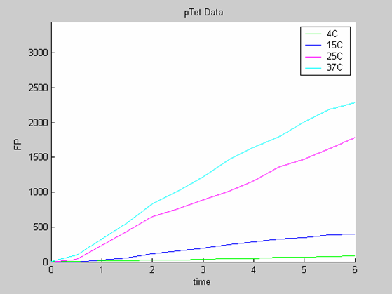
| - | + | [[Image:IC07_CFSpTet.png|left|thumb|400px|<font size=-2>'''Experimental data for pTet promoter in cell-free extract''' The time is expressed in hours. The concentration of Fluorescent Protein (GFP here) is in nanomol/l | |
| - | + | </font>]] | |
| - | + | ||
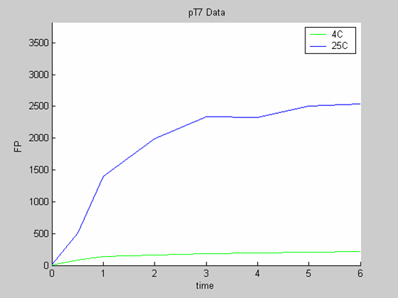
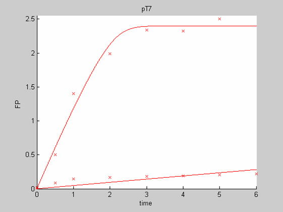
| - | + | [[Image:IC07_CFSpT7.png|none|thumb|400px|<font size=-2>'''Experimental data for pT7 promoter in cell-free extract''' The time is expressed in hours. The concentration of Fluorescent Protein (GFP here) is in nanomol/l | |
| - | | | + | </font>]] |
| - | '' | + | |
| - | ' | + | |
| Line 38: | Line 54: | ||
The differential equation governing the evolution of X , the concentration of GFP is | The differential equation governing the evolution of X , the concentration of GFP is | ||
| - | [[Image:IC07_CFSeqn1.png|center | + | [[Image:IC07_CFSeqn1.png|center]] |
In all cases the initial concentration of GFP was X<sub>0</sub> = 0. The solution of the equation is known explicitly. It is | In all cases the initial concentration of GFP was X<sub>0</sub> = 0. The solution of the equation is known explicitly. It is | ||
| - | [[Image:IC07_CFSeqn2.png|center | + | [[Image:IC07_CFSeqn2.png|center]] |
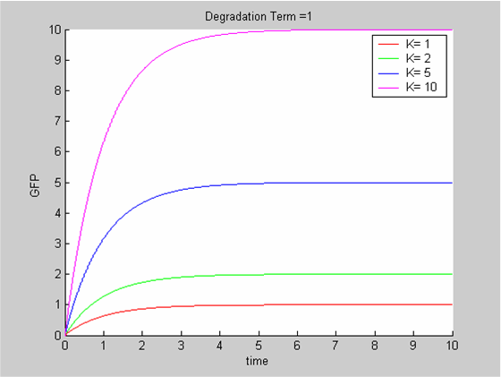
| - | + | [[Image:IC07_CFSdeg1.png|left|thumb|400px|<font size=-2>Solutions of the Classic ODE model for various values of the synthesis rate K (the degradation term is kept constant at 1)</font>]] | |
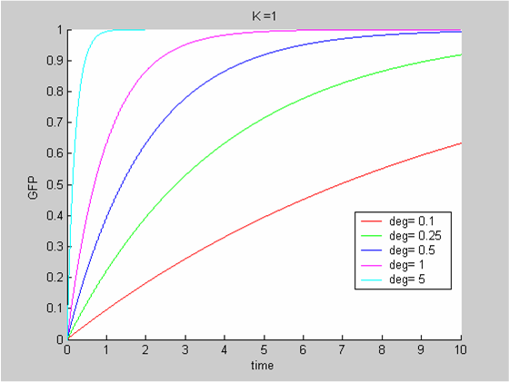
| - | + | [[Image:IC07_CFSk1.png|none|thumb|400px|<font size=-2>Solutions of the Classic ODE model for various values of the degradation term (the synthesis rate K is kept constant at 1)</font>]] | |
| - | + | ||
| - | + | ||
| - | + | ||
| Line 57: | Line 70: | ||
We let the time scale of the system (which is the chassis-dependent degradation term δ) run over a range of possible values and then we adjusted for each experiment the amplitude scale (the synthesis rate K) so the interpolation error was minimal for the experiment. The time scale (and the K’s) corresponding to the smallest overall error were then returned. | We let the time scale of the system (which is the chassis-dependent degradation term δ) run over a range of possible values and then we adjusted for each experiment the amplitude scale (the synthesis rate K) so the interpolation error was minimal for the experiment. The time scale (and the K’s) corresponding to the smallest overall error were then returned. | ||
| - | |||
==== Analysis 1 ==== | ==== Analysis 1 ==== | ||
We first analysed both promoter datasets (the pTet dataset and the pT7) independently. As can be seen below the model provides a good fit for each dataset. | We first analysed both promoter datasets (the pTet dataset and the pT7) independently. As can be seen below the model provides a good fit for each dataset. | ||
| - | + | [[Image:IC07_CFSpTet1.png|left|thumb|400px|<font size=-2>Interpolation of the PTet Data on their own. he time is expressed in hours. The concentration of Fluorescent Protein (GFP here) is in nanomol/l</font>]] | |
| - | + | [[Image:IC07_CFSpT71.png|none|thumb|400px|<font size=-2>Interpolation of the PT7 Data on their own. he time is expressed in hours. The concentration of Fluorescent Protein (GFP here) is in nanomol/l</font>]] | |
| - | + | ||
| - | + | ||
| - | + | ||
| - | The degradation term of the chassis was estimated to be 0.004/hour with the pTet data, which is consistent with statements of the manufacturer of the cell-free extract. However the pT7 data yield a very high degradation term (0.7/hour). The difference is high enough to suggest that the cause of such a variation is not rooted in the variability between two batches of cell extract. | + | |
| + | The degradation term of the chassis was estimated to be 0.004/hour with the pTet data, which is consistent with statements of the manufacturer of the cell-free extract. However the pT7 data yield a very high degradation term (0.7/hour). The difference is high enough to suggest that the cause of such a variation is not rooted in the variability between two batches of cell extract. | ||
==== Analysis 2 ==== | ==== Analysis 2 ==== | ||
When we analyse both datasets together the classic model yields a poor fit to our data as it fails to reconcile the linear behaviour of the pTet data with that of pT7 at 25 degrees (see images below). The estimated degradation is also high (degradation term = 0.24167) | When we analyse both datasets together the classic model yields a poor fit to our data as it fails to reconcile the linear behaviour of the pTet data with that of pT7 at 25 degrees (see images below). The estimated degradation is also high (degradation term = 0.24167) | ||
| - | + | [[Image:IC07_CFSpTet2.png|left|thumb|400px|<font size=-2>Interpolation of the PTet Data in conjonction with pT7. The time is expressed in hours. The concentration of Fluorescent Protein (GFP here) is in nanomol/l</font>]] | |
| - | + | [[Image:IC07_CFSpT72.png|none|thumb|400px|<font size=-2>Interpolation of the PT7 Data in conjonction with pTet. The time is expressed in hours. The concentration of Fluorescent Protein (GFP here) is in nanomol/l</font>]] | |
| - | + | ||
| - | + | ||
| - | | | + | |
| - | + | ||
| - | + | ||
| - | |||
| - | |||
==== Conclusion ==== | ==== Conclusion ==== | ||
The results of the data analysis with the classic model strongly '''suggest that the classic model is ill adapted to the description of protein synthesis in our cell free chassis. ''' | The results of the data analysis with the classic model strongly '''suggest that the classic model is ill adapted to the description of protein synthesis in our cell free chassis. ''' | ||
| + | == Temperature Dependence of the Synthesis Rate == | ||
| + | {| | ||
| + | |- | ||
| + | | | ||
| + | [[Image:CBD Arrhenius Plot.PNG|center|500px]] | ||
| + | [[Image:CellByDateArrhenius.png|center]]<br> | ||
| + | [[Image:CellByDateArrheniusPlot.png|center]] | ||
| + | |To elucidate the relationship between synthesis rate and temperature we thought to use the Arrhenius equation shown to the left which in our case would express the rate of protein synthesis as an exponential function.<br><br> | ||
| + | For Data analysis we would take logs of plot sides and do a log plot with data from isothermal experiments, calculating the Activation Energy (Ea) via division of the slope of the log plot by the universal gas constant.<br><br> | ||
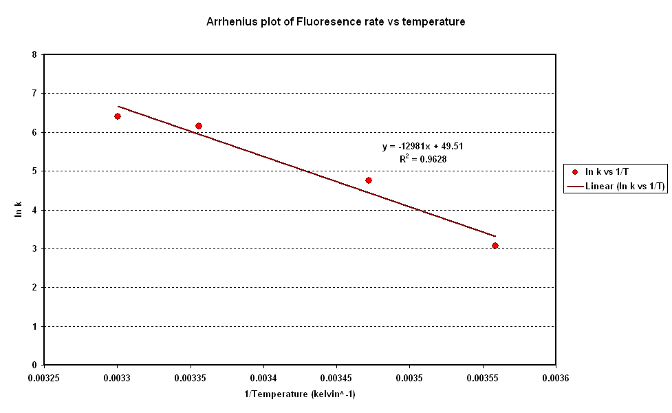
| + | For a range of isothermal scenarios for a pTET promoter [https://2007.igem.org/Imperial/Wet_Lab/Results/CBD2.2 (data here)] we extracted the rate of synthesis of GFP and plotted it against 1/T.<br><br> | ||
| + | A strong linear correlation in the log plot supports an arrhenius type dependence on temperature with an activation energy of 1.5kJ/mol. | ||
| + | In short there seems to be a similar relationship between temperature and synthesis rate.<br><br> | ||
| + | A more in depth analysis of these results can be found here as part of the[https://2007.igem.org/Imperial/Wet_Lab/Results/CBD2.2 cell by date project]. | ||
| + | |} | ||
== A Resource Dependent Model == | == A Resource Dependent Model == | ||
| - | The classic model cannot reconcile for the same degradation term a linear behaviour and a saturated behaviour. Several publications on systems expressing in cell-free extracts have shown that the lifespan of such systems was shorter than their counterparts in vivo and also that synthesis of proteins declined with time as the system ran out of resources. | + | The classic model cannot reconcile for the same degradation term a linear behaviour and a saturated behaviour. Several publications<sup>[[#References|1-2]]</sup> on systems expressing in cell-free extracts have shown that the lifespan of such systems was shorter than their counterparts in vivo and also that synthesis of proteins declined with time as the system ran out of resources. |
Such behaviour matches what we can observe for pT7 at 25 degrees. The concentration of GFP climbs steeply but this fast synthesis of GFP exhausts fast the resources of the system. Consequently synthesis grinds to a halt. Since the degradation term is very small in cell free extracts the concentration of GFP remains stable (instead of dropping). | Such behaviour matches what we can observe for pT7 at 25 degrees. The concentration of GFP climbs steeply but this fast synthesis of GFP exhausts fast the resources of the system. Consequently synthesis grinds to a halt. Since the degradation term is very small in cell free extracts the concentration of GFP remains stable (instead of dropping). | ||
| Line 95: | Line 112: | ||
We expand the classic model by introducing a function μ that quantifies the limiting effect of the resources available E on the synthesis of GFP. | We expand the classic model by introducing a function μ that quantifies the limiting effect of the resources available E on the synthesis of GFP. | ||
| - | [[Image:IC07_CFSeqn3.png|center | + | [[Image:IC07_CFSeqn3.png|center]] |
The more GFP is synthesized the faster the resources drop. We modelled this drop with a linear relation between the resources consumed and the amount of GFP synthesized. We call the ratio a the cost. | The more GFP is synthesized the faster the resources drop. We modelled this drop with a linear relation between the resources consumed and the amount of GFP synthesized. We call the ratio a the cost. | ||
Hence | Hence | ||
| - | [[Image:IC07_CFSeqn4.png|center | + | [[Image:IC07_CFSeqn4.png|center]] |
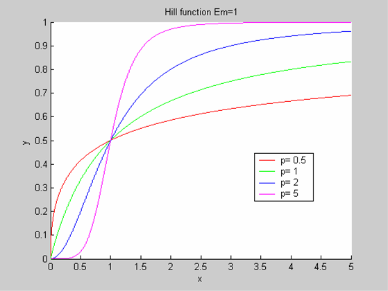
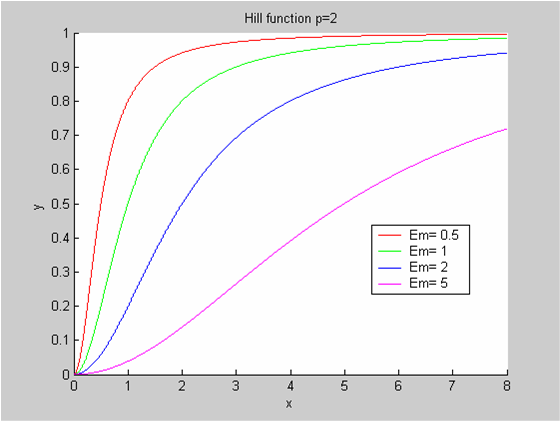
We chose to model the effect μ of the resources available on the synthesis of GFP with a Hill-Function of parameters Em and p. Em is the switching point of the function. The exponent p>=1 determines how steep the switching point is. | We chose to model the effect μ of the resources available on the synthesis of GFP with a Hill-Function of parameters Em and p. Em is the switching point of the function. The exponent p>=1 determines how steep the switching point is. | ||
| Line 106: | Line 123: | ||
* Conversely when resources are very low, μ is almost zero and synthesis grinds to a halt. | * Conversely when resources are very low, μ is almost zero and synthesis grinds to a halt. | ||
| - | [[Image:IC07_CFSeqn5.png|center | + | [[Image:IC07_CFSeqn5.png|center]] |
===== Images of Hill Graphs ===== | ===== Images of Hill Graphs ===== | ||
| - | + | [[Image:IC07_CFSh1.png|left|thumb|400px|<font size=-2>Allure of the Hill function for various values of the Exponent p</font>]] | |
| - | + | [[Image:IC07_CFSh2.png|none|thumb|400px|<font size=-2>Allure of the Hill function for various values of the switching point Em</font>]] | |
| - | + | ||
| - | + | ||
| - | + | ||
Thanks to the scaling properties of the Hill function, our model can be simplified and the chassis-dependent parameter can be eliminated from our model. Indeed it is not the variable E that determines the value of the Resource term μ but the ratio R=E/Em. | Thanks to the scaling properties of the Hill function, our model can be simplified and the chassis-dependent parameter can be eliminated from our model. Indeed it is not the variable E that determines the value of the Resource term μ but the ratio R=E/Em. | ||
The evolution of R is governed by the differential equation | The evolution of R is governed by the differential equation | ||
| - | [[Image:IC07_CFSeqn6.png|center | + | [[Image:IC07_CFSeqn6.png|center]] |
where the relative cost α directly relates to the cost a (α=a/ Em). | where the relative cost α directly relates to the cost a (α=a/ Em). | ||
Our resource-dependent model therefore is: | Our resource-dependent model therefore is: | ||
| - | [[Image:IC07_CFSeqn7.png|center | + | [[Image:IC07_CFSeqn7.png|center]] |
| - | Its initial conditions are [[Image:IC07_CFSeqn8.png | + | Its initial conditions are [[Image:IC07_CFSeqn8.png]] at t = 0 |
In this resource-dependent model, | In this resource-dependent model, | ||
| Line 139: | Line 154: | ||
The nice properties of the solution of the ODE system with no degradation terms allowed us to restrain the subspace of parameters that needed browsing and to develop an algorithm based on shape matching. | The nice properties of the solution of the ODE system with no degradation terms allowed us to restrain the subspace of parameters that needed browsing and to develop an algorithm based on shape matching. | ||
| - | More details on the algorithm we used to analyse the data and estimate the parameters of the model can be found in this complementary documentation | + | More details on the algorithm we used to analyse the data and estimate the parameters of the model can be found in this complementary documentation. |
| - | Results below show the best match that we could obtain for a Hill function of | + | Results below show the best match that we could obtain for a Hill function of exponent 1. |
| + | For and ODE system whose concentrations are expressed in micromol/l, the following results were obtained: | ||
| - | + | '''Initial Energy: 8''' | |
| - | + | '''Cost: 3.3333''' | |
| - | + | ||
| - | + | ||
| - | + | ||
| - | + | ||
| - | + | ||
| - | + | ||
| - | '''Initial Energy:8''' | + | |
| - | '''Cost:3.3333''' | + | |
'''pT7:''' | '''pT7:''' | ||
| Line 163: | Line 171: | ||
K(25 degrees) = 0.34667 | K(25 degrees) = 0.34667 | ||
K(37 degrees) = 0.49333 | K(37 degrees) = 0.49333 | ||
| + | |||
| + | '''Please note''' that this time the concentrations are in micromol/l. This change of scale was imposed on us by the ODE45 solver of Matlab that became unstable for the range of values we had to consider (very low α) | ||
| + | |||
| + | |||
| + | |||
| + | [[Image:IC07_CFSpT73.png|left|thumb|400px|<font size=-2>Interpolation of the PTet Data in conjunction with pT7 with the Resource dependent model. The time is expressed in hours. The concentration of Fluorescent Protein (GFP here) is in nanomol/l</font>]] | ||
| + | [[Image:IC07_CFSpTet3.png|left|thumb|400px|<font size=-2>Interpolation of the PT7 Data in conjunction with pTet with the Resource dependent model. The time is expressed in hours. The concentration of Fluorescent Protein (GFP here) is in nanomol/l</font>]] | ||
== Available Resources == | == Available Resources == | ||
| - | During this summer we have developed many routines with Matlab which we are happy to share with the rest of Synthetic Biology Community. They can be found in the | + | During this summer we have developed many routines with Matlab which we are happy to share with the rest of Synthetic Biology Community. They can be found in the [[Imperial/Dry_Lab/Software|Software Suite]] of the [[Imperial/Dry_Lab|Dry Lab]]. |
The applications that are most relevant to the chassis characterisation are | The applications that are most relevant to the chassis characterisation are | ||
* '''Constitutive Promoter Analysis''' | * '''Constitutive Promoter Analysis''' | ||
| - | Tag a constitutive promoter with a fluorescent protein, record the flurorescence and voila! | + | Tag a constitutive promoter with a fluorescent protein, record the flurorescence and voila! This routine loads the data as an excel sheet, allows you to visualize them and if need be to eliminate some samples you do not like. Then the synthesis rate and degradation term of the milieu are estimated. The routine was developed so the user may supervise all the operations. |
* '''Chassis Characterisation with the Classic Promoter Model''' | * '''Chassis Characterisation with the Classic Promoter Model''' | ||
The routine allows you to load the results of several experiments at the same time. These data are then analysed as described in section 3. Once the best fit is identified, the results are returned and the corresponding graphs are plotted. | The routine allows you to load the results of several experiments at the same time. These data are then analysed as described in section 3. Once the best fit is identified, the results are returned and the corresponding graphs are plotted. | ||
| - | + | == References == | |
| - | + | ||
| + | #Kim DM, Swartz JR. Prolonging Cell-Free Protein Synthesis with a Novel ATP Regeneration System. Biotechnology and Bioengineering, 1999. 66,3:181-188. | ||
| + | #Kim TW, Oh IS, Keum JW, Kwon YC, Byun JY, Lee KH, Choi CY, Kim DM. Prolonged Cell-Free Protein Synthesis Using Dual Energy Sources: Combined Use of Creatine Phosphate and Glucose for the Efficient Supply of ATP and Retarded Accumulation of Phosphate. Biotechnology and Bioengineering, 2007. 97,6:1510-1515 | ||
| + | |||
| - | + | <center> [https://2007.igem.org/Imperial/Cell-Free/Contribution << Our Contributions] | Characterisation | [https://2007.igem.org/Imperial/Cell-Free/Applications Applications >>] | |
| + | </center> | ||
Latest revision as of 01:10, 27 October 2007

Cell-Free: Characterisation
Introduction
In this section we analyse the data we have obtained on the cell-free chassis using GFP as the reporter. We show that the classic model for the synthesis of a protein by a constitutive promoter is not adapted and introduce a new model where synthesis is curbed by the resources left in the system. We also introduce an Arrhenius vision of the temperature dependence of sysnthesis rate. Finally we estimate the parameters of this new model from our data and show that it yields a much better fit.
Prior Knowledge
- pTet and pT7 are constitutive promoters that are commonly used in vivo for E. coli
- Tests in vitro have demonstrated that they also work on the cell-free chassis
- Manufacturer specifications: the solution has been optimised so the degradation of proteins is minimal. We therefore expect our analysis to find very small degradation terms
Available Data
We need as many data as possible and also data that are as varied as possible (data with similar behaviour will lead to the selection of a model that is too simple to predict all the behaviours that can be generated by the chassis).
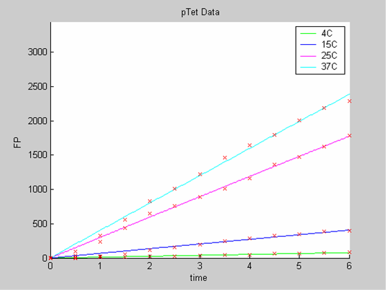
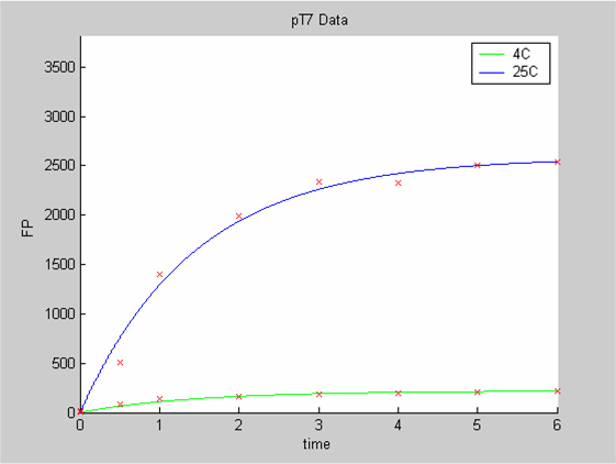
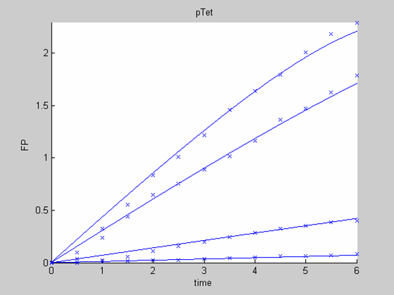
For this section we will use
- the data collected with pTet at 4,15,25 and 37 degrees that exhibit a linear behaviour
- the pT7 data at 4 and 25 degrees that exhibit a saturated behaviour.
We use the calibration curve of GFP to convert the fluorescence data into concentrations (in this case the concentrations were express in nanomols/l).
The Classic Model
To analyse our data we use the classic approach that consists of modelling the evolution with time of the concentrations of the product of interest. In this case the model is the simplest we can imagine:
- We have only one protein GFP
- It is constitutively synthesized at a constant synthesis rate K. K depends on the promoter that is used and ourdata show that it is also temperature-dependent
- The protein is then degraded. This degradation term δ depends on the protein and on the chassis. We can assume the impact of temperature to be negligible.
The differential equation governing the evolution of X , the concentration of GFP is
In all cases the initial concentration of GFP was X0 = 0. The solution of the equation is known explicitly. It is
Principle of our Data Analysis
Instead of analysing each experiment in isolation (for instance pTet at 25 degrees), we used several experiments in coordination. The idea was to force our data analysis routine to return only one degradation term for the whole series of experiment (since the degradation term is chassis-dependent) and one synthesis rate per experiment (the rate K is promoter and temperature dependent, that is in our case experiment-dependent).
The algorithm we developed for our data analysis used the scaling properties of the solutions of the differential equations. We let the time scale of the system (which is the chassis-dependent degradation term δ) run over a range of possible values and then we adjusted for each experiment the amplitude scale (the synthesis rate K) so the interpolation error was minimal for the experiment. The time scale (and the K’s) corresponding to the smallest overall error were then returned.
Analysis 1
We first analysed both promoter datasets (the pTet dataset and the pT7) independently. As can be seen below the model provides a good fit for each dataset.
The degradation term of the chassis was estimated to be 0.004/hour with the pTet data, which is consistent with statements of the manufacturer of the cell-free extract. However the pT7 data yield a very high degradation term (0.7/hour). The difference is high enough to suggest that the cause of such a variation is not rooted in the variability between two batches of cell extract.
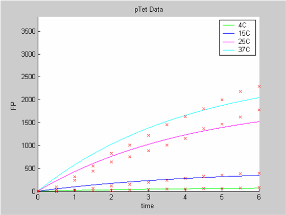
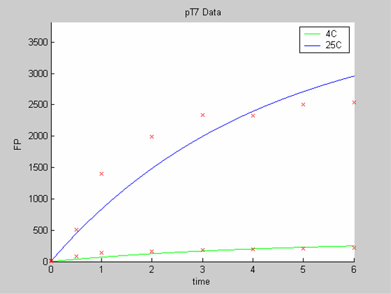
Analysis 2
When we analyse both datasets together the classic model yields a poor fit to our data as it fails to reconcile the linear behaviour of the pTet data with that of pT7 at 25 degrees (see images below). The estimated degradation is also high (degradation term = 0.24167)
Conclusion
The results of the data analysis with the classic model strongly suggest that the classic model is ill adapted to the description of protein synthesis in our cell free chassis.
Temperature Dependence of the Synthesis Rate
|
| To elucidate the relationship between synthesis rate and temperature we thought to use the Arrhenius equation shown to the left which in our case would express the rate of protein synthesis as an exponential function. For Data analysis we would take logs of plot sides and do a log plot with data from isothermal experiments, calculating the Activation Energy (Ea) via division of the slope of the log plot by the universal gas constant. |
A Resource Dependent Model
The classic model cannot reconcile for the same degradation term a linear behaviour and a saturated behaviour. Several publications1-2 on systems expressing in cell-free extracts have shown that the lifespan of such systems was shorter than their counterparts in vivo and also that synthesis of proteins declined with time as the system ran out of resources.
Such behaviour matches what we can observe for pT7 at 25 degrees. The concentration of GFP climbs steeply but this fast synthesis of GFP exhausts fast the resources of the system. Consequently synthesis grinds to a halt. Since the degradation term is very small in cell free extracts the concentration of GFP remains stable (instead of dropping).
We expand the classic model by introducing a function μ that quantifies the limiting effect of the resources available E on the synthesis of GFP.
The more GFP is synthesized the faster the resources drop. We modelled this drop with a linear relation between the resources consumed and the amount of GFP synthesized. We call the ratio a the cost. Hence
We chose to model the effect μ of the resources available on the synthesis of GFP with a Hill-Function of parameters Em and p. Em is the switching point of the function. The exponent p>=1 determines how steep the switching point is.
- If the model has enough resources E>>Em then μ is almost 1 and the synthesis of GFP proceeds unhinged.
- Conversely when resources are very low, μ is almost zero and synthesis grinds to a halt.
Images of Hill Graphs
Thanks to the scaling properties of the Hill function, our model can be simplified and the chassis-dependent parameter can be eliminated from our model. Indeed it is not the variable E that determines the value of the Resource term μ but the ratio R=E/Em.
The evolution of R is governed by the differential equation
where the relative cost α directly relates to the cost a (α=a/ Em).
Our resource-dependent model therefore is:
Its initial conditions are  at t = 0
In this resource-dependent model,
- K is promoter and temperature dependent.
- α, R0 and δ are chassis dependent.
Simulations and Results
See Cell by Date.
Data Analysis
We tried to estimate the characteristics of the chassis according to our new model. In order to save some computation-time we made the assumption that the degradation terms were negligible (the pTet data and the manufacturer’s claims back this up).
The nice properties of the solution of the ODE system with no degradation terms allowed us to restrain the subspace of parameters that needed browsing and to develop an algorithm based on shape matching. More details on the algorithm we used to analyse the data and estimate the parameters of the model can be found in this complementary documentation.
Results below show the best match that we could obtain for a Hill function of exponent 1. For and ODE system whose concentrations are expressed in micromol/l, the following results were obtained:
Initial Energy: 8 Cost: 3.3333
pT7: K (4 degrees) = 0.053333 K (25 degrees) = 1.3867
pTet: K(4 degrees) = 0.013333 K (15 degrees) = 0.08 K(25 degrees) = 0.34667 K(37 degrees) = 0.49333
Please note that this time the concentrations are in micromol/l. This change of scale was imposed on us by the ODE45 solver of Matlab that became unstable for the range of values we had to consider (very low α)
Available Resources
During this summer we have developed many routines with Matlab which we are happy to share with the rest of Synthetic Biology Community. They can be found in the Software Suite of the Dry Lab.
The applications that are most relevant to the chassis characterisation are
- Constitutive Promoter Analysis
Tag a constitutive promoter with a fluorescent protein, record the flurorescence and voila! This routine loads the data as an excel sheet, allows you to visualize them and if need be to eliminate some samples you do not like. Then the synthesis rate and degradation term of the milieu are estimated. The routine was developed so the user may supervise all the operations.
- Chassis Characterisation with the Classic Promoter Model
The routine allows you to load the results of several experiments at the same time. These data are then analysed as described in section 3. Once the best fit is identified, the results are returned and the corresponding graphs are plotted.
References
- Kim DM, Swartz JR. Prolonging Cell-Free Protein Synthesis with a Novel ATP Regeneration System. Biotechnology and Bioengineering, 1999. 66,3:181-188.
- Kim TW, Oh IS, Keum JW, Kwon YC, Byun JY, Lee KH, Choi CY, Kim DM. Prolonged Cell-Free Protein Synthesis Using Dual Energy Sources: Combined Use of Creatine Phosphate and Glucose for the Efficient Supply of ATP and Retarded Accumulation of Phosphate. Biotechnology and Bioengineering, 2007. 97,6:1510-1515
